Arzela-Ascoli Theorem and Applications

The Arzela-Ascoli Theorem is a rather formidable-sounding theorem that gives a necessary and sufficient condition for a sequence of real-valued continuous functions on a closed and bounded interval to have a uniformly convergent subsequence.

Statement: Let $(f_n)$ be a uniformly bounded and equicontinuous sequence of real-valued continuous functions defined on a closed and bounded interval $[a,b]$ . Then there exists a subsequence $(f_{n_k})$ that converges uniformly.

The converse of the Arzela-Ascoli Theorem is also true, in the sense that if every subsequence of $(f_n)$ has a uniformly convergent subsequence, then $(f_n)$ is uniformly bounded and equicontinuous.

Explanation of terms used: A sequence $(f_n)$ of functions on $[a,b]$ is uniformly bounded if there is a number $M$ such that $|f_n(x)|\leq M$ for all $f_n$ and all $x\in [a,b]$ . The sequence is equicontinous if, for all $\epsilon>0$ , there exists $\delta>0$ such that $|f_n(x)-f_n(y)|<\epsilon$ whenever $|x-y|<\delta$ for all functions $f_n$ in the sequence. The key point here is that a single $\delta$ (depending solely on $\epsilon$ ) works for the entire family of functions.

Application

Let $g:[0,1]\times [0,1]\to [0,1]$ be a continuous function and let $\{f_n\}$ be a sequence of functions such that $f_n(x)=\begin{cases}0,&0\leq x\leq 1/n\\ \int_0^{x-\frac{1}{n}}g(t,f_n(t))\ dt,&1/n\leq x\leq 1\end{cases}$

Prove that there exists a continuous function $f:[0,1]\to\mathbb{R}$ such that $f(x)=\int_0^x g(t,f(t))\ dt$ for all $x\in [0,1]$ .

The idea is to use Arzela-Ascoli Theorem. Hence, we need to show that $(f_n)$ is uniformly bounded and equicontinuous.

We have

$\begin{aligned}|f_n(x)|&\leq |\int_0^{x-\frac{1}{n}} 1\ dt|\\ &=|x-\frac{1}{n}|\\ &\leq |x|+|\frac{1}{n}|\\ &\leq 1+1\\ &=2 \end{aligned}$

This shows that the sequence is uniformly bounded.

If $0\leq x\leq 1/n$ ,

$\begin{aligned}|f_n(x)-f_n(y)|&=|0-f_n(y)|\\ &=|\int_0^{y-\frac{1}{n}} g(t,f_n(t))\ dt|\\ &\leq |\int_0^{y-\frac{1}{n}} 1\ dt|\\ &=|y-\frac{1}{n}|\\ &\leq |y-x| \end{aligned}$

Similarly if $0\leq y\leq 1/n$ , $|f_n(x)-f_n(y)|\leq |x-y|$ .

If $1/n\leq x\leq 1$ and $1/n\leq y\leq 1$ ,

$\begin{aligned}|f_n(x)-f_n(y)|&=|\int_0^{x-1/n} g(t,f_n(t))\ dt-\int_0^{y-1/n}g(t,f_n(t))\ dt|\\ &=|\int_{y-1/n}^{x-1/n}g(t,f_n(t))\ dt|\\ &\leq |\int_{y-1/n}^{x-1/n} 1\ dt|\\ &=|(x-1/n)-(y-1/n)|\\ &=|x-y| \end{aligned}$

Therefore we may choose $\delta=\epsilon$ , then whenever $|x-y|<\delta$ , $|f_n(x)-f_n(y)|\leq |x-y|<\epsilon$ . Thus the sequence is indeed equicontinuous.

By Arzela-Ascoli Theorem, there exists a subsequence $(f_{n_k})$ that is uniformly convergent.

$f_{n_k}(x)\to f(x)=\int_0^x g(t,f(t))\ dt$ .

By the Uniform Limit Theorem, $f:[0,1]\to\mathbb{R}$ is continuous since each $f_n$ is continuous.

Quotient Ring of the Gaussian Integers is Finite

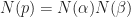
The Gaussian Integers $\mathbb{Z}[i]$ are the set of complex numbers of the form $a+bi$ , with $a,b$ integers. Originally discovered and studied by Gauss, the Gaussian Integers are useful in number theory, for instance they can be used to prove that a prime is expressible as a sum of two squares iff it is congruent to 1 modulo 4.

This blog post will prove that every (proper) quotient ring of the Gaussian Integers is finite. I.e. if $I$ is any nonzero ideal in $\mathbb{Z}[i]$ , then $\mathbb{Z}[i]/I$ is finite.

We will need to use the fact that $\mathbb{Z}[i]$ is an Euclidean domain, and thus also a Principal Ideal Domain (PID).

Thus $I=(\alpha)$ for some nonzero $\alpha\in\mathbb{Z}[i]$ . Let $\beta\in\mathbb{Z}[i]$ .

By the division algorithm, $\beta=\alpha q+r$ with $r=0$ or $N(r)<N(\alpha)$ . We also note that $\beta+I=r+I$ .

Thus,

$\begin{aligned}\mathbb{Z}[i]/I&=\{\beta+I\mid\beta\in\mathbb{Z}[i]\}\\ &=\{r+I\mid r\in\mathbb{Z}[i],N(r)<N(\alpha)\} \end{aligned}$ .

Since there are only finitely many elements $r\in\mathbb{Z}[i]$ with $N(r)<N(\alpha)$ , thus $\mathbb{Z}[i]/I$ is finite.

Behavior of Homotopy Groups with respect to Products

This blog post is on the behavior of homotopy groups with respect to products. Proposition 4.2 of Hatcher:

For a product $\prod_\alpha X_\alpha$ of an arbitrary collection of path-connected spaces $X_\alpha$ there are isomorphisms $\pi_n(\prod_\alpha X_\alpha)\cong\prod_\alpha \pi_n(X_\alpha)$ for all $n$ .

The proof given in Hatcher is a short one: A map $f:Y\to \prod_\alpha X_\alpha$ is the same thing as a collection of maps $f_\alpha: Y\to X_\alpha$ . Taking $Y$ to be $S^n$ and $S^n\times I$ gives the result.

A possible alternative proof is to first prove that $\pi_n(X_1\times X_2)\cong\pi_n(X_1)\times\pi_n(X_2)$ , which is the result for a product of two spaces. The general result then follows by induction.

We construct a map $\psi:\pi_n(X_1\times X_2)\to\pi_n(X_1)\times\pi_n(X_2)$ , $\psi([f])=([f_1],[f_2])$ .

Notation: $f:S^n\to X_1\times X_2$ , $f_1=p_1\circ f:S^n\to X_1$ , $f_2=p_2\circ f:S^n\to X_2$ where $p_i:X_1\times X_2\to X_i$ are the projection maps.

We can show that $\psi ([f]+[g])=\psi([f])+\psi([g])$ , thus $\psi$ is a homomorphism.

We can also show that $\psi$ is bijective by constructing an explicit inverse, namely $\phi:\pi_n(X_1)\times\pi_n(X_2)\to\pi_n(X_1\times X_2)$ , $\phi([g_1],[g_2])=[g]$ where $g:S^n\to X_1\times X_2$ , $g(x)=(g_1(x),g_2(x))$ .

Thus $\psi$ is an isomorphism.

Graph of measurable function is measurable (and has measure zero)

Let $f$ be a finite real valued measurable function on a measurable set $E\subseteq\mathbb{R}$ . Show that the set $\{(x,f(x)):x\in E\}$ is measurable.

We define $\Gamma(f,E):=\{(x,f(x)):x\in E\}$ . This is popularly known as the graph of a function. Without loss of generality, we may assume that $f$ is nonnegative. This is because we can write $f=f^+ - f^-$ , where we split the function into two nonnegative parts.

The proof here can also be found in Wheedon’s Analysis book, Chapter 5.

The strategy for proving this question is to approximate the graph of the function with arbitrarily thin rectangular strips. Let $\epsilon>0$ . Define $E_k=\{x\in E\mid \epsilon k\leq f(x)<\epsilon (k+1)\}$ , $k=0,1,2,\dots$ .

Also, $\Gamma(f,E)=\cup\Gamma(f,E_k)$ , where $\Gamma(f,E_k)$ are disjoint.

$\begin{aligned}|\Gamma(f,E)|_e&\leq\sum_{k=1}^\infty|\Gamma(f,E_k)|_e\\ &\leq\epsilon(\sum_{k=1}^\infty|E_k|)\\ &=\epsilon|E| \end{aligned}$

If $|E|<\infty$ , we can conclude $|\Gamma(f,E)|_e=0$ and thus $\Gamma(f,E)$ is measurable (and has measure zero).

If $|E|=\infty$ , we partition $E$ into countable union of sets $F_k$ each with finite measure. By the same analysis, each $\Gamma(f,F_k)$ is measurable (and has measure zero). Thus $\Gamma(f,E)=\bigcup_{k=1}^\infty\Gamma(f,F_k)$ is a countable union of measurable sets and thus is measurable (has measure zero).

Mean Value Theorem for Higher Dimensions

Let $f$ be differentiable on a connected set $E\subseteq \mathbb{R}^n$ , then for any $x,y\in E$ , there exists $z\in E$ such that $f(x)-f(y)=\nabla f(z)\cdot (x-y)$ .

Proof: The trick is to use the Mean Value Theorem for 1 dimension via the following construction:

Define $g:[0,1]\to\mathbb{R}$ , $g(t)=f(tx+(1-t)y)$ . By the Mean Value Theorem for one variable, there exists $c\in (0,1)$ such that $g'(c)=\frac{g(1)-g(0)}{1-0}$ , i.e.

$\nabla f(cx+(1-c)y)\cdot (x-y)=f(x)-f(y)$ . Here we are using the chain rule for multivariable calculus to get: $g'(c)=\nabla f(cx+(1-c)y)\cdot (x-y)$ .

Let $z=cx+(1-c)y$ , then $\nabla f(z)\cdot (x-y)=f(x)-f(y)$ as required.

Every non-empty open set in R is disjoint union of countable collection of open intervals

Question: Prove that every non-empty open set in $\mathbb{R}$ is the disjoint union of a countable collection of open intervals.

The key things to prove are the disjointness and the countability of such open intervals. Otherwise, if disjointness and countability are not required, we may simply take a small open interval centered at each point in the open set, and their union will be the open set.

Elementary Proof: Let $U$ be a non-empty open set in $\mathbb{R}$ .

Let $x\in U$ . There exists an open interval $I\subseteq U$ containing $x$ . Let $I_x$ be the maximal open interval in $U$ containing $x$ , i.e. for any open interval $I\subseteq U$ containing $x$ , $I\subseteq I_x$ . (The existence of $I_x$ is guaranteed, we can take it to be the union of all open intervals $I\subseteq U$ containing $x$ .)

We note that such maximal intervals are equal or disjoint: Suppose $I_x\cap I_y\neq\emptyset$ and $I_x\neq I_y$ then $I_x\cup I_y$ is an open interval in $U$ containing $x$ , contradicting the maximality of $I_x$ .

Each of the maximal open intervals contain a rational number, thus we may write $\displaystyle U=\bigcup_{q\in U\cap\mathbb{Q}}I_q$ . Upon discarding the “repeated” intervals in the union above, we get that $U$ is the disjoint union of a countable collection of open intervals.

There are many other good proofs of this found here (http://math.stackexchange.com/questions/318299/any-open-subset-of-bbb-r-is-a-at-most-countable-union-of-disjoint-open-interv), though some can be quite deep for this simple result.

Useful Theorem in Introductory Ring Theory

Something interesting I realised in my studies in Math is that certain theorems are more “useful” than others. Certain theorems’ sole purpose seem to be an intermediate step to prove another theorem and are never used again. Other theorems seem to be so useful and their usage is everywhere.

One of the most “useful” theorems in basic Ring theory is the following:

Let $R$ be a commutative ring with 1 and $I$ an ideal of $R$ . Then

(i) $I$ is prime iff $R/I$ is an integral domain.

(ii) $I$ is maximal iff $R/I$ is a field.

With this theorem, the following question is solved effortlessly:

Let $R$ be a commutative ring with 1 and let $I$ and $J$ be ideals of $R$ such that $I\subseteq J$ .

(i) Show that $J$ is a prime ideal of $R$ iff $J/I$ is a prime ideal of $R/I$ .

(ii) Show that $J$ is a maximal ideal of $R$ iff $J/I$ is a maximal ideal of $R/I$ .

Sketch of Proof of (i):

$J$ is a prime ideal of $R$ iff $R/J$ is an integral domain. ( $R/J\cong \frac{R/I}{J/I}$ by the Third Isomorphism Theorem. ) $\iff$ $J/I$ is a prime ideal of $R/I$ .

(ii) is proved similarly.

Fundamental Group of Torus (van Kampen method)

There are various methods of computing fundamental groups, for example one method using maximal trees of a simplicial complex (considered a slow method). There is one “trick” using van Kampen’s Theorem that makes it relatively fast to compute the fundamental group.

This “trick” doesn’t seem to be explicitly written in books, I had to search online to learn about it.

Fundamental Group of Torus

First we let $U$ and $V$ be open subsets of the torus (denoted as $X$ )as shown in the diagram below. $U$ is an open disk, while $V$ is the entire space with a small punctured hole. We are using the fundamental polygon representation of the torus. This trick can work for many spaces, not just the torus.

$U$ is contractible, thus $\pi_1(U)=0$ . $U\cap V$ has $S^1$ as a deformation retract, thus $\pi_1(U\cap V)=\mathbb{Z}$ . We note that $X=U\cup V$ and $U\cap V$ is path-connected. These are the necessary conditions to apply van Kampen’s Theorem.

Then, by Seifert-van Kampen Theorem, $\displaystyle\boxed{\pi_1(X)=\pi_1(U)\coprod_{\pi_1(U\cap V)}\pi_1(V)}$ , the free product of $\pi_1(U)$ and $\pi_1(V)$ with amalgamation.

Let $h$ be the generator in $U\cap V$ . We have $j_{1*}(h)=1$ and $j_{2*}(h)=aba^{-1}b^{-1}$ . ( $j_1:U\cap V\to U$ and $j_2:U\cap V\to V$ are the inclusions. )

Therefore

$\begin{aligned} \pi_1(X)&=\langle a,b\mid aba^{-1}b^{-1}=1\rangle\\ &=\langle a,b\mid ab=ba\rangle\\ &\cong\mathbb{Z}\times\mathbb{Z} \end{aligned}$

vankampen_torus

Free Math Newsletter

Interpolation Technique in Analysis

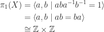
Question: Let $f$ belong to both $L^{p_1}$ and $L^{p_2}$ , with $1\leq p_1<p_2<\infty$ . Show that $f\in L^p$ for all $p_1\leq p\leq p_2$ .

There is a pretty neat trick to do this question, known as the “interpolation technique”. The proof is as follows.

For $p_1<p<p_2$ , there exists $0<\alpha<1$ such that $\displaystyle\boxed{p=\alpha p_1+(1-\alpha)p_2}$ . This is the key “interpolation step”. Once we have this, everything flows smoothly with the help of Holder’s inequality.

$\displaystyle\begin{aligned} \int |f|^p\ d\mu&=\int (|f|^{\alpha p_1}\cdot |f|^{(1-\alpha)p_2})\ d\mu\\ &\leq\||f|^{\alpha p_1}\|_\frac{1}{\alpha}\||f|^{(1-\alpha)p_2}\|_\frac{1}{1-\alpha}\\ &=(\int |f|^{p_1}\ d\mu)^\alpha\cdot (\int |f|^{p_2}\ d\mu)^{1-\alpha}\\ &<\infty \end{aligned}$

Thus $f\in L^p$ .

Note that the magical thing about the interpolation technique is that $p=\frac{1}{\alpha}$ and $q=\frac{1}{1-\alpha}$ are Holder conjugates, since $\frac{1}{p}+\frac{1}{q}=1$ is easily verified.

Undergraduate Math Books

Interesting Measure and Integration Question

Let $(\Omega,\mathcal{A},\mu)$ be a measure space. Let $f\in L^p$ and $\epsilon>0$ . Prove that there exists a set $E\in\mathcal{A}$ with $\mu(E)<\infty$ , such that $\int_{E^c} |f|^p<\epsilon$ .

Solution:

The solution strategy is to use simple functions (common tactic for measure theory questions).

Let $0\leq\phi\leq |f|^p$ be a simple function such that $\int_\Omega (|f|^p-\phi)\ d\mu<\epsilon$ .

Consider the set $E=\{\phi>0\}$ . Note that $\int_\Omega \phi\ d\mu\leq\int_\Omega |f|^p\ d\mu<\infty$ . Hence each nonzero value of $\phi$ can only be on a set of finite measure. Since $\phi$ has only finitely many values, $\mu(E)<\infty$ .

Then,

$\begin{aligned} \int_{E^c}|f|^p\ d\mu&=\int_{E^c} (|f|^p-\phi)\ d\mu +\int_{E^c}\phi\ d\mu\\ &\leq \int_\Omega (|f|^p-\phi)\ d\mu+0\\ &<\epsilon \end{aligned}$

Z(D_2n), Center of Dihedral Group D_2n

Click here for Free Personality Test

Question: What is $Z(D_{2n})$ , the center of the dihedral group $D_{2n}$ ?

Algebraically, the dihedral group may be viewed as a group with two generators $a$ and $b$ , i.e. $\boxed{D_{2n}=\{1,a,a^2,\dots,a^{n-1},b,ab,a^2b,\dots,a^{n-1}b\}}$ with $a^n=b^2=1$ , $bab=a^{-1}$ .

Answer: $Z(D_2)=D_2$

$Z(D_4)=D_4$ .

For $n\geq 3$ , $Z(D_{2n})=\begin{cases}1&,\ n\ \text{is odd}\\ \{1,a^{n/2}\}&,\ n\ \text{is even} \end{cases}$

Proof: For $n=1$ , $D_2=\{1, b\}\cong\mathbb{Z}_2$ which is abelian. Thus, $Z(D_2)=D_2$ .

For $n=2$ , $D_4=\{1,a,b,ab\}\cong V$ , the Klein four-group, which is also abelian. Thus, $Z(D_4)=D_4$ .

Let $A=\{1,a,a^2,\dots,a^{n-1}\}$ , $B=\{b,ab,a^2b,\dots,a^{n-1}b\}$ . Clearly elements in $A$ commute with each other.

Let $a^k$ be an element in $A$ . ( $0\leq k\leq n-1$ ). Let $a^lb$ be an element in $B$ . ( $0\leq l\leq n-1$ )

$\begin{aligned}a^k(a^lb)=(a^lb)a^k&\iff a^kb=ba^k\\ &\iff a^kba^{-k}b^{-1}=1\\ &\iff a^kb(bab)^kb=1\ (\text{here we used}\ bab=a^{-1})\\ &\iff a^kb(ba^kb)b=1\\ &\iff a^{2k}=1\\ &\iff k=0\ \text{or}\ n/2 \end{aligned}$

I.e. the only element in $A$ (other than 1) that is in the center is $a^{n/2}$ , which is only possible if $n$ is even.

Let $a^kb$ , $a^lb$ be two distinct elements in $B$ . ( $0\leq k< l\leq n-1$ )

$\begin{aligned}(a^kb)(a^lb)=(a^lb)(a^kb)&\iff ba^l=a^{l-k}ba^k\\ &\iff ba^{l-k}=a^{l-k}b \end{aligned}$

By earlier analysis, this is true iff $l-k=n/2$ . Each $a^kb\ (0\leq k\leq n-2)$ is not in the center since we may consider $l=k+1$ , i.e. $a^{k+1}b$ . Then $l-k=1<n/2$ . (since $n\geq 3$ ). $a^{n-1}b$ also does not commute with $a^{n-2}b$ for the same reason.

Therefore,

For $n\geq 3$ , $Z(D_{2n})=\begin{cases}1&,\ n\ \text{is odd}\\ \{1,a^{n/2}\}&,\ n\ \text{is even} \end{cases}$

Projective Space Explicit Homotopy (RP1 to RP2)

Free Career Personality Quiz

The above video describes the real projective plane ( $\mathbb{R}P^2$ ).

The projective space $\mathbb{R}P^n$ can be defined as the quotient space of $S^n$ by the equivalence relation $x\sim -x$ for $x\in S^n$ .

Notation: For $x=(x_1,\dots, x_{n+1})\in S^n$ , we write $[x_1, x_2,\dots, x_{n+1}]$ for the corresponding point in $\mathbb{R}P^n$ . Let $f,g: \mathbb{R}P^1\to\mathbb{R}P^2$ be the maps defined by $f[x,y]=[x,y,0]$ and $g[x,y]=[x,-y,0]$ .

How do we construct an explicit homotopy between $f$ and $g$ ? A common mistake is to try the “straight-homotopy”, e.g. $F([x,y],t)=[x,(1-2t)y,0]$ . This is a mistake as it passes through the point [0,0,0] which is not part of the projective plane.

A better approach is to consider $F:\mathbb{R}P^1\times I\to\mathbb{R}P^2$ , defined by $\boxed{F([x,y],t)=[x,(\cos\pi t)y, (\sin\pi t)y]}$ .

Note that if $x^2+y^2=1$ , then $x^2+[(\cos\pi t)y]^2+[(\sin\pi t)y]^2=x^2+y^2=1$ .

$F([x,y],0)=[x,y,0]$

$F([x,y],1)=[x,-y,0]$

Calculus World Cup

Just to share this news:

The National Taiwan University is holding the first ever Calculus World Cup (CWC) in February 2016. It’s the first time students from global top universities will be able to compete over Calculus in e-sports. The competition will be held on PaGamO – a social online gaming platform for education. The top 12 teams will be invited to Taiwan for the final round, and great prizes with a value of over $70,000 await the finalists!
Official website: http://cwc.pagamo.com.tw

Registration: https://pagamo.com.tw/calculus_cup

Facebook: https://www.facebook.com/PaGamo.glo

Outer measure of Symmetric Difference Zero implies Measurability

Free Career Quiz: Please help to do!

Just came across this neat beginner’s Lebesgue Theory question. As students of analysis know, just to show a set is measurable is no easy feat. The usual way is to use the Caratheodory definition, where a set E is said to be measurable if for any set A, $m^*(A)=m^*(A\cap E)+m^*(A\cap E^c)$ . This can be quite tedious.

Question: Suppose E is a Lebesgue measurable set and let F be any subset of $\mathbb{R}$ such that $m^*(E\Delta F)=0$ (Symmetric Difference is Zero). Show that F is measurable.

The short way to do this is to note that $m^*(E\Delta F)=0$ implies $m^*(E\setminus F)=0$ , and $m^*(F\setminus E)=0$ . This in turn (using a lemma that any set with outer measure zero is measurable) implies the measurability of $E\setminus F$ and $\setminus F\setminus E$ .

Next comes the critical observation: $\boxed{E\cap F=E\setminus (E\setminus F)=E\cap (E\setminus F)^c}$ . Using the fact that the collection of measurable sets is a $\sigma$ -algebra, we can conclude $E\cap F$ is measurable.

Thus $F=(E\cap F)\cup (F\setminus E)$ is the union of two measurable sets and thus is measurable.

Interesting indeed!

Fermat’s Two Squares Theorem (Gaussian Integers approach)

Today we will discuss Fermat’s Two Squares Theorem using the approach of Gaussian Integers, the set of numbers of the form a+bi, where a, b are integers. This theorem is also called Fermat’s Christmas Theorem, presumably because it is proven during Christmas.

Have you ever wondered why $5=1^2+2^2$ , $13=2^2+3^2$ can be expressed as a sum of two squares, while not every prime can be? This is no coincidence, as we will learn from the theorem below.

Theorem: An odd prime p is the sum of two squares, i.e. $p=a^2+b^2$ where a, b are integers if and only if $p\equiv 1 \pmod 4$ .

(=>) The forward direction is the easier one. Note that $a^2\equiv 0\pmod 4$ if a is even, and $a^2\equiv 1\pmod 4$ if a is odd. Similar for b. Hence $p=a^2+b^2$ can only be congruent to 0, 1 or 2 (mod 4). Since p is odd, this means $p\equiv 1\pmod 4$ .

(<=) Conversely, assume $p\equiv 1\pmod 4$ , where p is a prime. p=4k+1 for some integer k.

First we prove a lemma called Lagrange’s Lemma: If $p\equiv 1\pmod 4$ is prime, then $p\mid (n^2+1)$ for some integer n.

Proof: By Wilson’s Theorem, $(p-1)!=(4k)!\equiv -1\pmod p$ . $(4k)!\equiv [(2k)!]^2\equiv -1\pmod p$ . We may see this by observing that $4k\equiv p-1\equiv -1\pmod p$ , $4k-1\equiv -2\pmod p$ , …, $4k-(2k-1)=2k+1\equiv -2k\pmod p$ . Thus $[(2k)!]^2+1\equiv 0\pmod p$ and hence $p\mid n^2+1$ , where $n=(2k)!$ .

Then $p\mid (n+i)(n-i)$ . However $p\nmid (n+i)$ since $p\nmid n=(2k)!$ . Similarly, $p\nmid (n-i)$ . Therefore $p$ is not a Gaussian prime, and it is thus not irreducible.

$p=\alpha\beta$ with $N(\alpha)>1$ and $N(\beta)>1$ . $N(p)=N(\alpha)N(\beta)$ , which means $p^2=N(\alpha)N(\beta)$ . Thus we may conclude $N(\alpha)=p$ , $N(\beta)=p$ .

Let $\alpha=a+bi$ . Then $p=a^2+b^2$ and we are done.

This proof is pretty amazing, and shows the connection between number theory and ring theory.

Holder’s Inequality Trick

Click here: Free Career Quiz

Holder’s Inequality is a very useful inequality in Functional Analysis, hence many results can be proved by applying Holder’s Inequality.

Suppose that $\mu(\Omega)<\infty$ and $1\leq p_1<p_2\leq\infty$ . Prove that if $f_n\to f$ in $L^{p_2}$ , then $f_n\to f$ in $L^{p_1}$ .

Proof: Assume $f_n\to f$ in $L^{p_2}$ . Then there exists $N$ such that if $n\geq N$ , then $\|f_n-f\|_{p_2}=(\int |f_n-f|^{p_2} d\mu)^{1/p_2}<\epsilon$ .

Then, $\begin{aligned} \|f_n-f\|_{p_1}^{p_1}&=\int |f_n-f|^{p_1} d\mu\\ &=\||f_n-f|^{p_1}\cdot 1\|_1\\ &\leq\||f_n-f|^{p_1}\|_{p_2/p_1}\|1\|_{(p_2/p_1)'},\ \ \ \text{where } (p_2/p_1)'=\frac{p_2}{p_2-p_1}\ \text{is the Holder conjugate}\\ &=(\int |f_n-f|^{p_2}d\mu)^{p_1/p_2}(\int 1 d\mu)^\frac{p_2-p_1}{p_2}\\ &<\epsilon^{p_1}\cdot \mu(\Omega)^\frac{p_2-p_1}{p_2} \end{aligned}$

Since $\epsilon>0$ is arbitrary, $\|f_n-f\|_{p_1}^{p_1}\to 0$ as $n\to\infty$ .

Therefore, $\|f_n-f\|_{p_1}\to 0$ .

mu is countably additive if and only if it satisfies the Axiom of Continuity

Free Career Personality Quiz (Hundreds of people have tried it!)

Let $\mu$ be a finite, non-negative, finitely additive set function on a measurable space $(\Omega, \mathcal{A})$ . Show that $\mu$ is countably additive if and only if it satisfies the Axiom of Continuity: For $E_n\in\mathcal{A}, E_n\downarrow\emptyset \implies \mu(E_n)\to 0$ .

(=>) Assume $\mu$ is countably additive. Let $E_n\in\mathcal{A}$ , $E_n\downarrow\emptyset$ . Then,

$\displaystyle \lim_n \mu (E_n)=\mu (\cap_{n=1}^\infty E_n)=\mu (\emptyset)$ .

Suppose $\mu(\emptyset)=c$ . Then $\mu(\emptyset)=\mu(\cup_{n=1}^\infty \emptyset)=\sum_{n=1}^\infty c$ implies $c=0$ .

(<=) Assume $\mu$ satisfies Axiom of Continuity. Let $A_n\in\mathcal{A}$ be mutually disjoint sets. Define $E_n=\cup_{i=1}^\infty A_i\setminus \cup_{i=1}^n A_i$ .

Then $E_n\downarrow\emptyset$ . $\lim_n \mu(E_n)=0$ , $\lim_n \mu(\cup_{i=1}^\infty A_i)-\mu (\cup_{i=1}^n A_i)=0$ . $\lim_n \mu(\cup_{i=1}^n A_i)=\mu (\cup_{i=1}^\infty A_i)$ .

Therefore

$\begin{aligned}\mu(\cup_{i=1}^\infty A_i)&=\lim_n \mu(\cup_{i=1}^n A_i)\\ &=\lim_n \sum_{i=1}^n \mu (A_i)\\ &=\sum_{i=1}^\infty \mu(A_i) \end{aligned}$

Measure that is absolutely continuous with respect to mu

Interesting Career Personality Test (Free): https://mathtuition88.com/free-career-quiz/

Let $(X,\mathcal{M},\mu)$ be a measure space, and let $f:X\to [0,\infty]$ be a measurable function. Define the map $\lambda:\mathcal{M}\to[0,\infty]$ , $\lambda(E):=\int_X \chi_E f d\mu$ , where $\chi_E$ denotes the characteristic function of $E$ .

(a) Show that $\lambda$ is a measure and that it is absolutely continuous with respect to $\mu$ .

(b) Show that for any measurable function $g:X\to[0,\infty]$ , one has $\int_X g d\lambda=\int_X gf d\mu$ in $[0,\infty]$ .

Proof: For part (a), we routinely check that $\lambda$ is indeed a measure.

$\lambda(\emptyset)=\int_X \chi_\emptyset f d\mu=\int_X 0 d\mu=0$ . Let $E_i$ be mutually disjoiint measurable sets.

$\begin{aligned} \lambda(\cup_{i=1}^\infty E_i)&=\int_X \chi_{\cup_{i=1}^\infty E_i} f d\mu\\ &=\int_X (\sum_{i=1}^\infty \chi_{E_i}) f d\mu\\ &=\sum_{i=1}^\infty \int_X \chi_{E_i} f d\mu\\ &=\sum_{i=1}^\infty \lambda (E_i) \end{aligned}$

If $\mu (E)=0$ , then $\chi_{E} f=0$ a.e., thus $\lambda (E)=0$ . Therefore $\lambda\ll\mu$ .

(b) We note that when $g$ is a characteristic function, i.e. $g=\chi_E$ ,

$\begin{aligned} \int_X g d\lambda&=\int_X \chi_E d\lambda\\ &=\lambda (E)\\ &=\int_X \chi_E f d\mu\\ &=\int_X gf d\mu \end{aligned}$

Hence the equation holds. By linearity, we can see that the equation holds for all simple functions. Let $(\psi_n)$ be a sequence of simple functions such that $\psi_n\uparrow g$ . Then by the Monotone Convergence Theorem, $\lim_{n\to\infty} \int \psi_n d\lambda=\int g d\lambda$ .

Note that $\psi_n f\uparrow gf$ , thus by MCT, $\lim_{n\to\infty}\int\psi_n f d\mu=\int g f d\mu$ . Note that $\int \psi_n d\lambda=\int \psi_n f d\mu$ . Hence, $\int g d\lambda=\int gf d\mu$ , and we are done.

f integrable implies set where f is infinite is measure zero

Let $(X,\mathcal{M},\mu)$ be a measure space. Let $f:X\to [0,\infty]$ be a measurable function. Suppose that $\int_X f d\mu<\infty$ .

(a) Show that the set $\{x\in X:f(x)=\infty\}\subseteq X$ is of $\mu$ -measure 0. (Intuitively, this is quite obvious, but we need to prove it rigorously.)

(b) Show that the set $\{x\in X:f(x)\neq 0\}\subseteq X$ is $\sigma$ -finite with respect to $\mu$ . i.e. it is a countable union of measurable sets of finite $\mu$ -measure.

We may use Markov’s inequality, which turns out to be very useful in this question.

Proof: (a) Let $E_k=\{x\in X:f(x)\geq k\}$ , where $k\in\mathbb{N}$ . Denote $E_\infty=\{x\in X:f(x)=\infty\}$ .

$E_K \downarrow E_\infty$ , and $\mu (E_1)\leq\frac{1}{1}\int_X f d\mu<\infty$ . (Markov Inequality!)

Then

$\begin{aligned}\mu(E_\infty)&=\lim_{k\to\infty}\mu (E_k)\\ &\leq\lim_{k\to\infty}\frac{1}{k}\int f d\mu\ \ \ \text{(Markov Inequality)}\\ &=0 \end{aligned}$

Therefore, $\mu(E_\infty)=0$ .

(b) Let $S_k=\{x\in X:f(x)\geq\frac{1}{k}\}$ , $k\in\mathbb{N}$ .

$\{x\in X:f(x)\neq 0\}=\cup_{k=1}^\infty S_k$

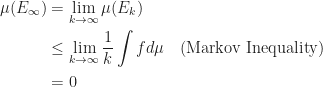
Therefore, $\mu(S_k)\leq k\int f d\mu<\infty$ , and we have expressed the set as a countable union of measurable sets of finite measure.

Once again, do check out the Free Career Quiz!

Interesting Analysis Question (Measure Theory)

Do try out this Free Career Guidance Personality Test at https://career-test.com/s/sgamb?reid=210 while it is still available!

Benefits of doing the (Free) Career Test:

Get familiar with the top companies in Singapore
There are seven distinct career types based on career preferences, goals and personality. Get to know yours! (My result: Harmonizer)
Take part in the annual Universum survey and win prizes!

Let $f\geq 0$ be a measurable function with $\int f d\mu<\infty$ . Show that for any $\epsilon>0$ , there exists a $\delta(\epsilon)>0$ such that for any measurable set $E\in\mathcal{A}$ with $\mu(E)<\delta(\epsilon)$ , we have $\int_E f d\mu<\epsilon$ .

Proof: For $M>0$ , we define $f_M(x)=\min (f(x),M)\leq M$ , for all $x\in \Omega$ .

Then $f=f_M+(f-f_M)$ .

Let $\delta=\epsilon/2M$ . Then for any $E\in\mathcal{A}$ with $\mu(E)<\delta$ ,

$\begin{aligned}\int_E f_M d\mu &\leq \int_E M d\mu\\ &=\mu (E)M\\ &<\delta M\\ &=(\epsilon/2M)M\\ &=\epsilon/2 \end{aligned}$

Note that $f_M\uparrow f$ . By Monotone Convergence Theorem,

$\int f d\mu=\lim_{M\to\infty}\int f_M d\mu$ .

Therefore $\lim_{M\to\infty}\int f-f_M d\mu=0$ .

We can choose $M$ sufficiently large such that

$\int_E f-f_M d\mu \leq \int f-f_M d\mu <\epsilon/2$ .

Then

$\begin{aligned} \int_E f d\mu&=\int_E f_M d\mu+\int_E f-f_M d\mu\\ &<\epsilon/2+\epsilon/2\\ &=\epsilon \end{aligned}$

We are done!

Conjugacy Classes of non-abelian group of order p^3

Do try out this Free Career Guidance Personality Test at https://career-test.com/s/sgamb?reid=210 while it is still available!

Benefits of doing the (Free) Career Test:

Get familiar with the top companies in Singapore
There are seven distinct career types based on career preferences, goals and personality. Get to know yours! (My result: Harmonizer)
Take part in the annual Universum survey and win prizes!

Let p be a prime, and let G be a non-abelian group of order $p^3$ . We want to find the number of conjugacy classes of G.

First we prove a lemma: Z(G) has order p.

Proof: We know that since G is a non-trivial p-group, then $Z(G)\neq 1$ . Since $Z(G)\trianglelefteq G$ , by Lagrange’s Theorem, $|Z(G)|=p,p^2,\text{or }p^3$ .

Case 1) $|Z(G)|=p$ . We are done.

Case 2) $|Z(G)|=p^2$ . Then $|G/Z(G)|=p^3/p=p$ . Thus $G/Z(G)$ is cyclic which implies that G is abelian. (contradiction).

Case 3) $|Z(G)|=p^3$ . This means that the entire group G is abelian. (contradiction).

Next, let $O(x_1),\dots, O(x_n)$ be the distinct conjugacy classes of G.

$O(x_i)=\{gx_i g^{-1}:g\in G\}$ , where $C_G(x_i)=\{g\in G:gx_i=x_ig\}$ .

Then by the Class Equation, we have $\displaystyle p^3=|G|=\sum_{i=1}^n [G:C_G(x_i)]$ .

If $x_i\in Z(G)$ , then $C_G(x_i)=G$ , which means $[G:C_G(x_i)]=1$ .

If $x_i \notin Z(G)$ , then $C_G(x_i)\neq G$ . Since $x_i\in C_G(x_i)$ , thus $Z(G)\subsetneq C_G(x_i)$ . Thus we have $p=|Z(G)|<|C_G(x_i)|<|G|=p^3$ . Since $C_G(x_i)$ is a subgroup of $G$ , Lagrange’s Theorem forces $|C_G(x_i)|=p^2$ . Thus $[G:C_G(x_i)]=p^3/p^2=p$ .

By the Class Equation, we thus have $p^3=p+(n-p)p$ , which leads us to $\boxed{n=p^2+p-1}$ .

Singapore Haze & Subgroup of Smallest Prime Index

Recently, the Singapore Haze is getting quite bad, crossing the 200 PSI Mark on several occasions. Do consider purchasing a Air Purifier, or some N95 Masks, as the haze problem is probably staying for at least a month. Personally, I use Nasal Irrigation (Neilmed Sinus Rinse), which has tremendously helped my nose during this haze period. It can help clear out dust and mucus trapped in the nose.

[S$89.90][Clean Air]2015 Air Purifier Singapore brand and 1 year warranty with HEPA Activated Carbon UV-C germicidal killer lamp silent operation and high efficiency etc

WWW.QOO10.SG

[S$19.90]Haze Prevention~ Nasal Rinse™- Flush out mucous~germs~bacteria~and dirt internally. Clear blocked nose and very soothing.

WWW.QOO10.SG

Previously, we proved that any subgroup of index 2 is normal. It turns out that there is a generalisation of this theorem. Let $p$ be the smallest prime divisor of a group $G$ . Then, any subgroup $H\leq G$ of index $p$ is normal in $G$ .

Proof: Let $H$ be a subgroup of $G$ of index $p$ . Let $G$ act on the left cosets of $H$ by left multiplication: $\forall x\in G$ , $x\cdot gH=xgH$ .

This group action induces a group homomorphism $\phi:G\to S_p$ .

Let $K=\ker \phi$ . If $x\in K$ , then $xgH=gH$ for all $g\in G$ . In particular when g=1, xH=H, i.e. $x\in H$ .

Thus $K\subseteq H$ . In particular, $K\trianglelefteq H$ , since $\ker\phi$ is a normal subgroup of $G$ .

We have $G/K\cong \phi(G)\leq S_p$ . Thus $|G/K|\mid p!$ .

Also note that $|G|=|G/K||K|$ . Note that $|G/K|\neq 1$ since $|G/K|=[G:H][H:K]=p[H:K]\geq p$ .

Let $q$ be a prime divisor of $|G/K|$ . Then $q\leq p$ since $|G/K|\mid p!$ . Also, $q\mid |G|$ . Since $p$ is the smallest prime divisor of $|G|$ , $p\leq q$ . Therefore, $p=q$ , i.e. $|G/K|=p$ .

Then $p=p[H:K] \implies [H:K]=1$ , i.e. H=K. Thus, H is normal in G.

Zmn/Zm isomorphic to Zn

The following is a simple proof of why $\mathbb{Z}_{mn}/\mathbb{Z}_m\cong\mathbb{Z}_n$ .

For instance $\mathbb{Z}_6/\mathbb{Z}_2\cong\mathbb{Z}_3$ . Note that the tricky part is that $\mathbb{Z}_2$ is not actually the usual {0,1}, but rather {0,3} (considered as part of $\mathbb{Z}_6$ ). Hence the elements of $\mathbb{Z}_6/\mathbb{Z}_2$ are {0,3}, {1, 4}, {2, 5}, which can be seen to be isomorphic to $\mathbb{Z}_3$ .

A sketch of a proof is as follows. Consider $\phi:\mathbb{Z}_{mn}/\mathbb{Z}_m\to \mathbb{Z}_n$ , where $\mathbb{Z}_m=\{0,n,2n,\dots,(m-1)n\}$ , defined by $\phi (a+\mathbb{Z}_m)=a$ .

We may check that it is well-defined since if $a+\mathbb{Z}_m=a'+\mathbb{Z}_m$ , then $a\equiv a' \pmod n$ , and thus $\phi (a+\mathbb{Z}_m)=\phi (a'+\mathbb{Z}_m)$ .

It is a fairly straightforward to check it is a homomorphism, $\begin{aligned}\phi (a+\mathbb{Z}_m+a'+\mathbb{Z}_m)&=\phi (a+a'+\mathbb{Z}_m)\\ &=a+a'\\ &=\phi (a+\mathbb{Z}_m)+\phi(a'+\mathbb{Z}_m) \end{aligned}$

Injectivity is clear since $\ker \phi=0+\mathbb{Z}_m$ , and surjectivity is quite clear too.

Hence, this ends the proof. 🙂

Do check out some Recommended Books on Undergraduate Mathematics, and also download the free SG50 Scientific Pioneers Ebook, if you haven’t already.

Free Ebook: Singapore’s Scientific Pioneers

Source: http://www.asianscientist.com/pioneers/

The non-commercial book Singapore’s Scientific Pioneers, sponsored by grants from the SG50 Celebration Fund and Nanyang Technological University, is dedicated to all scientists in Singapore, past, present and, most of all, aspiring. Read more from Asian Scientist Magazine at: http://www.asianscientist.com/pioneers/

The free downloadable book also includes a Mathematician from National University of Singapore, Professor Louis Chen, one of the discoverers of the Chen-Stein method.

To download the ebook, click here to download (official mirror).

The Chen-Stein method is part of the branch of Mathematics known as Probability. Advanced probability requires a lot of Measure Theory, another type of Math classified under Analysis.

In the book, Professor Chen mentioned one of his favourite books is “One Two Three . . . Infinity: Facts and Speculations of Science (Dover Books on Mathematics)“.

It turns out that this book is very inspiring, and many reviewers on Amazon said that after they read this book during their childhood, they became inspired to become mathematicians/scientists!

Sample review (from Amazon): “It seems that almost all the reviewers had the same experience: we read this book at an early age, and it was so fascinating, so inspiring, and so magical that it directed us into math and science for the rest of our lives. In my case the book was loaned to me when I was about 12, by my best friend’s father.”

Hence, if you are looking for a Math/Science book for your child, this book may be one of the top choices. 🙂

Weierstrass M-test Proof and Special Case of Abel’s Theorem

First, let us recap what is Weierstrass M-test:

Weierstrass M-test:

Let $\{f_n\}$ be a sequence of real (or complex)-valued functions defined on a set A, and let $\{M_n\}$ be a sequence satisfying $\forall n\in\mathbb{N}, \forall x\in A$

$|f_n (x)|\leq M_n$ , and also $\sum_{n=1}^\infty M_n=M<\infty$ .

Then, $\sum_{n=1}^\infty f_n(x)$ converges uniformly on A (to a function f).

Proof:

Let $\epsilon >0$ . $\exists N\in\mathbb{N}$ such that $m\geq N$ implies $|M-\sum_{n=1}^m M_n|<\epsilon$ .

For $m\geq N, \forall x\in A$ ,

$\begin{aligned} |f(x)-\sum_{n=1}^m f_n(x)|&=|\sum_{n=m+1}^\infty f_n (x)|\\ &\leq\sum_{n=m+1}^\infty |f_n (x)|\\ &\leq \sum_{n=m+1}^\infty M_n\\ &=|M-\sum_{n=1}^m M_n|\\ &<\epsilon \end{aligned}$

Thus, $\sum_{n=1}^\infty f_n (x)$ converges uniformly.

Application to prove Abel’s Theorem (Special Case):

Consider the special case of Abel’s Theorem where all the coefficients $a_i$ are of the same sign (e.g. all positive or all negative).

Then, for $x\in [0,1]$ ,

$|a_n x^n|\leq |a_n|:=M_n$

Then by Weierstrass M-test, $\sum_{n=1}^\infty a_n x^n$ converges uniformly on [0,1] and thus $\lim_{x\to 1^-} \sum_{n=1}^\infty a_n x^n=\sum_{n=1}^\infty a_n$ .

Check out some books suitable for Math Majors here!

Allot more time for exam papers (Straits Times Forum)

Source: http://www.straitstimes.com/forum/letters-on-the-web/allot-more-time-for-exam-papers

This reader has called for allotting more time for exam papers. He/she has made a very valid point:

The time allotted for some papers, such as mathematics, is so limited that the opportunity cost of stopping for just a few minutes to think about how to solve a problem may result in one being unable to complete the paper.

For essay papers in subjects such as economics, it becomes a test of how fast one can write, as opposed to the quality of one’s answers.

This is very true, the reader is being 100% honest and not exaggerating at all! For O Levels and A Levels Maths, the student can only spend 1.5min per mark. That means, for a 5 mark long question, he can only spend 7.5 min at the maximum or risk not being able to finish the paper. To have ample time to check the paper, the student needs to do even faster than the minimum of 1.5 min per mark.

Yoda’s quote “Do. Or do not. There is no try.” holds true for Mathematics exam papers in Singapore. There is simply no time to “try” out questions in O Level or A Level Maths. Once a student looks at the question, his fate is sealed, he/she either knows the method how to do it, or does not. There is no time to try!

Hence, exam time management skills and speed in Math are essential. (I have written a previous post about it.) Nowadays, questions are not arranged in order of difficulty. This means that Question 5 may be much harder than Question 10. Sometimes, it is better to skip Question 5, rather than get stuck on it and never reach Question 10. Getting 100% is not necessary for getting an A for Math. In fact, getting 100% for Math after Primary 6 is a rare occurrence. Getting 70 for Math in H2 Math is a very decent score, and getting 80 more or less guarantees an A even with a bell curve.

Also, knowledge of the essential formulas are extremely important. Yes, it is possible to derive the quadratic formula by completing the square, but there is no time for that during the exam. Time is of essence. Formula for AP/GP, Vectors need to be known by heart. Spending 1 min to recall or derive them may lead to severe time pressure later on. Recalling the wrong formula leads to disaster, and potentially zero marks for the entire question, as “error carry forward” is only applicable for limited scenarios. Students may need a Formula Helpsheet containing all the essential formulas for easy memorization.

Lastly, the most important thing the night before the exam is have a good night’s sleep. A previous blog post discusses the importance of sleep, and how Good night’s sleep adds up to better exam results – especially in maths. Also, have a good rest after the Math paper, the 3 hour H2 paper is mentally exhausting, and the 2.5 hour A Maths paper is not a stroll in the park either. After the long Maths paper, your brain deserves a good rest.

Proof of Associativity of Operation * on Path-homotopy Classes

(Continued from https://mathtuition88.com/2015/06/25/the-groupoid-properties-of-operation-on-path-homotopy-classes-proof/)

Earlier we have proved the properties (2) Right and left identities, (3) Inverse, leaving us with (1) Associativity to prove.

For this proof, it will be convenient to describe the product f*g in the language of positive linear maps.

First we will need to define what is a positive linear map. We will elaborate more on this since Munkres’ books only discusses it briefly.

Definition: If [a,b] and [c,d] are two intervals in $\mathbb{R}$ , there is a unique map $p:[a,b]\to [c.d]$ of the form p(x)=mx+k that maps a to c and b to d. This is called the positive linear map of [a,b] to [c,d] because its graph is a straight line with positive slope.

Why is it a positive slope? (Not mentioned in the book) It turns out to be because we have:

p(a) = ma+k=c

p(b) = mb+k=d

Hence, d-c = mb-ma = m(b-a)

Thus, m=(d-c)/(b-a), which is positive since d-c and b-a are all positive quantities.

Note that the inverse of a positive linear map is also a positive linear map, and the composite of two such maps is also a positive linear map.

Now, we can show that the product f*g can be described as follows: On [0,1/2], it is the positive linear map of [0,1/2] to [0,1], followed by f; and on [1/2,1] it equals the positive linear map of [1/2,1] to [0,1], followed by g.

Let’s see why this is true. The positive linear map of [0,1/2] to [0,1] is p(x)=2x. fp(x) = f(2x).

The positive linear map of [1/2,1] to [0,1] is p(x)=2x-1. gp(x)=g(2x-1).

If we look back at the earlier definition of f*g, that is precisely it!

Now, given paths, f, g, and h in X, the products f*(g*h) and (f*g)*h are defined if and only if f(1)=g(0) and g(1)=h(0), i.e. the end point of f = start point of g, and the end point of g = start point of h. If we assume that these two conditions hold, we can also define a triple product of the paths f, g, and h as follows:

Choose points a and b of I so that 0<a<b<1. Define a path $k_{a,b}$ in X as follows: On [0,a] it equals the positive linear map of [0,a] to I=[0,1] followed by f; on [a,b] it equals the positive linear map of [a,b] to I followed by g; on [b,1] it equals the positive linear map of [b,1] to I followed by h. This path $k_{a,b}$ depends on the choice of the values of a and b, but its path-homotopy class turns out to be independent of a and b.

We can show that if c and d are another pair of points of I with 0<c<d<1, then $k_{c,d}$ is path homotopic to $k_{a,b}$ .

Let $p:I\to I$ be the map whose graph is pictured in Figure 51.9 (taken from Munkre’s Book)

On the intervals [0,a], [a,b], [b,1], it equals the positive linear maps of these intervals onto [0,c],[c,d],[d,1] respectively. It follows that $k_{c,d} \circ p = k_{a,b}$ . Let’s see why this is so.

On [0,a] $k_{c,d}\circ p$ is the positive linear map of [0,a] to [0,c], followed by the positive linear map of [0,c] to I, followed by f. This equals the positive linear map of [0,a] to I, followed by f, which is precisely $k_{a,b}$ . Similar logic holds for the intervals [a,b] and [b,1].

$p$ is a path in I from 0 to 1, and so is the identity map $i: I\to I$ . Since I is convex, there is a path homotopy P in I between p and i. Then, $k_{c,d}\circ P$ is a path homotopy in X between $k_{a,b}$ and $k_{c.d}$ .

Now the question many will be asking is: What has this got to do with associativity. According to the author Munkres, “a great deal”! We check that the product $f*(g*h)$ is exactly the triple product $k_{a,b}$ in the case where $a=1/2$ and $b=3/4$ .

By definition,

$(g*h)(s)=\begin{cases} g(2s)\ &\text{for }s\in [0,\frac{1}{2}]\\ h(2s-1)\ &\text{for }s\in [\frac{1}{2},1] \end{cases}$

Thus, $f*(g*h)(s)=\begin{cases} f(2s)\ &\text{for }s\in [0,\frac{1}{2}]\\ (g*h)(2s-1)\ &\text{for }s\in [\frac{1}{2},1] \end{cases} =\begin{cases} f(2s)\ &\text{for }s\in [0,\frac{1}{2}]\\ g(4s-2)\ &\text{for }s\in [\frac{1}{2},\frac{3}{4}]\\ h(4s-3) &\text{for }s\in [\frac{3}{4},1] \end{cases}$

We can also check in a very similar way that $(f*g)*h)=k_{c,d}$ when c=1/4 and d=1/2. Thus, the these two products are path homotopic, and we have finally proven the associativity of *.

Reference:

Topology (2nd Economy Edition)

H2 Maths Distinction Rate (Percentage of As)

H2 Mathematics has one of the highest distinction rates of all subjects (around 50% each year). This means that around half of all Singaporean A level candidates score an A for H2 Maths!

H2 A Level Distinction Rates Compilation (National Average)

(For year 2010)

H2 Mathematics Distinction Rate: 51.9%
H2 Biology Distinction Rate: 43.7%
H2 Economics Distinction Rate: 33.8%

H1 Mathematics Distinction Rate: 33.1%
H1 Economics Distinction Rate: 33.8%

Literature Distinction Rate: 30.1%
History Distinction Rate: 23.7%
Geography Distinction Rate: 28.3%

Source: http://ajc.edu.sg/pdf/aj_broadcast/newsroom/news_archives/linkaj_may_2011.pdf

H2 Maths Notes and Resources

Check out the highly summarized and condensed H2 Maths Notes here! (Comes with Free H2 Math Exam Papers.)

Is H2 Maths the easiest H2 subject to get A?

Answer: Yes, provided the student does study conscientiously and not lag behind too much. Based on the statistics above, one can easily see that based on probability alone, H2 Maths is the easiest H2 subject to get A. Since more than 50% of students get A for H2 Maths, in a sense it is easier to get A for H2 Maths than flipping a heads on a coin!

However… (Please Read)

H2 Maths is also the easiest to fail! Without sufficient practice and effort to understand the subject material, sub-30 (below 30/100) marks are extremely common for H2 Maths. Last minute cramming will simply not work, and if a student lags too far behind in terms of syllabus, it will take extra effort to just even catch up.

In Depth Analysis of H2 Maths Distinction Rate

The 50% National Distinction Rate for H2 Maths can be quite misleading to think that every student has 50% chance of getting A for H2 Maths. The truth is that H2 Maths Distinction Rate varies a lot from school to school.

For example, AJC’s H2 Maths Distinction Rate is 62.7%, which is very much higher than the 50% average National Distinction Rate.

Raffles Institution (RI/RJC) Distinction Rate hovers around 70% to 80%!

Victoria JC (VJC)’s H2 Maths Distinction Rate is around 66.6%.

Hwa Chong (HCI) H2 Maths Distinction Rate is around 80% (8 out of 10 students scored an A for H2 Maths in HCI for three consecutive years).

Upon some thinking, one will quickly realize that if so many schools have Distinction Rate significantly above 50%, there has to be many schools with Distinction Rate significantly below 50%, in order for the National Distinction Rate to be around 50%!

The only people who know the exact Distinction Rate for the above mentioned JCs would be the internal staff and students, since the school website will probably not publish the statistics for obvious reasons.

The Best Time to Study H2 Maths is Now!

For students who are in schools with super high H2 Maths Distinction Rate, congratulations, your chances of getting A for H2 Maths are very good. However, do not be complacent till the very last day, as the race is not over yet.

For students who are in schools with very low H2 Maths Distinction Rate, the odds are unfortunately stacked against the student. However, do not lose heart, as anything is possible if one puts one’s heart and mind into it.

Good luck!

H2 Maths Notes and Resources

Check out the highly summarized and condensed H2 Maths Notes here! (Comes with Free H2 Math Exam Papers.)

H2 Math Tuition

https://mathtuition88.com/

“I LOVE YOU” Math Graph

This is how to plot “I LOVE YOU” using Math Graphs (many piecewise functions plotted together).

Interesting? Share it using the buttons below this post!

Source: Found it on Weibo (China’s version of Facebook)

Love and Math: The Heart of Hidden Reality

What if you had to take an art class in which you were only taught how to paint a fence? What if you were never shown the paintings of van Gogh and Picasso, weren’t even told they existed? Alas, this is how math is taught, and so for most of us it becomes the intellectual equivalent of watching paint dry.

In Love and Math, renowned mathematician Edward Frenkel reveals a side of math we’ve never seen, suffused with all the beauty and elegance of a work of art. In this heartfelt and passionate book, Frenkel shows that mathematics, far from occupying a specialist niche, goes to the heart of all matter, uniting us across cultures, time, and space.

What is a Measure? (Measure Theory)

In layman’s terms, “measures” are functions that are intended to represent ideas of length, area, mass, etc. The inputs for the measure functions would be sets, and the output would be a real value, possibly including infinity.

It would be desirable to attach the value 0 to the empty set $\emptyset$ and measures should be additive over disjoint sets in X.

Definition (from Bartle): A measure is an extended real-valued function $\mu$ defined on a $\sigma$ -algebra X of subsets of X such that
(i) $\mu (\emptyset)=0$
(ii) $\mu (E) \geq 0$ for all $E\in \mathbf{X}$
(iii) $\mu$ is countably additive in the sense that if $(E_n)$ is any disjoint sequence ( $E_n \cap E_m =\emptyset\ \text{if }n\neq m$ ) of sets in X, then

$\displaystyle \mu(\bigcup_{n=1}^\infty E_n )=\sum_{n=1}^\infty \mu (E_n)$ .

If a measure does not take on $+\infty$ , we say it is finite. More generally, if there exists a sequence $(E_n)$ of sets in X with $X=\cup E_n$ and such that $\mu (E_n) <+\infty$ for all n, then we say that $\mu$ is $\sigma$ -finite. We see that if a measure is finite implies it is $\sigma$ -finite, but not necessarily the other way around.

Examples of measures

(a) Let X be any nonempty set and let X be the $\sigma$ -algebra of all subsets of X. Let $\mu_1$ be definied on X by $\mu_1 (E)=0$ , for all $E\in\mathbf{X}$ . We can see that $\mu_1$ is finite and thus also $\sigma$ -finite.

Let $\mu_2$ be defined by $\mu_2 (\emptyset) =0$ , $\mu_2 (E)=+\infty$ if $E\neq \emptyset$ . $\mu_2$ is an example of a measure that is neither finite nor $\sigma$ -finite.

The most famous measure is definitely the Lebesgue measure. If X=R, and X=B, the Borel algebra, then (shown in Bartle’s Chapter 9) there exists a unique measure $\lambda$ defined on B which coincides with length on open intervals. I.e. if E is the nonempty interval (a,b), then $\lambda (E)=b-a$ . This measure is usually called Lebesgue measure (or sometimes Borel measure). It is not a finite measure since $\lambda (\mathbb{R})=\infty$ . But it is $\sigma$ -finite since any interval can be broken down into a sequence of sets ( $E_n$ ) such that $\mu (E_n)<\infty$ for all n.

Source: The Elements of Integration and Lebesgue Measure

A nonnegative function f in M(X,X) is the limit of a monotone increasing sequence in M(X,X)

We will elaborate on a lemma in the book The Elements of Integration and Lebesgue Measure.

Lemma: If f is a nonnegative function in M(X,X), then there exists a sequence ( $\phi_n$ ) in M(X,X) such that:

(a) $0\leq \phi_n (x) \leq \phi_{n+1} (x)$ for $x\in X, n\in\mathbb{N}$ .

(b) $f(x) =\lim \phi_n (x)$ for each $x\in X$ .

Proof:

Let n be a fixed natural number. If k=0, 1, 2, …, $n 2^n -1$ , let $E_{kn}$ be the set

$E_{kn}=\{ x\in X: k2^{-n} \leq f(x)<(k+1)2^{-n}\}$ .

If $k=n2^n$ , let $E_{kn}=\{x\in X: f(x) \geq n\}$ .

We note that the sets $\{E_{kn}: k=0, 1,\ldots, n2^n\}$ are disjoint.

The sets also belong to X, and have union equal to X.

Thus, if we define $\phi_n= k2^{-n}$ on $E_{kn}$ , then $\phi_n$ belongs to M(X,X).

We can see that the properties (a), (b), (c) hold.

(a): $0\leq k2^{-n}\leq k2^{-n-1}$ is true.

(I just noticed there is some typo in Bartle’s book, as the above inequality does not hold. I think n is supposed to be fixed, while k is increased instead.)

(b): As n tends to infinity, on $k2^{-n} \leq f(x) <(k+1)2^{-n}$ , i.e. $\phi_n (x) \leq f(x) < \phi_n (x)+2^{-n}$ , thus $f(x)=\lim \phi_n (x)$ for each $x\in X$ .

(c): Clearly true!

Source:

Coursera Probability Course and Recommended Probability Book

Just completed the Coursera Probability Course by UPenn (University of Pennsylvania), lectured by Professor Santosh S. Venkatesh who is the author of the highly recommended book: The Theory of Probability: Explorations and Applications.

Coursera Review

The course isn’t very hard, it is very suitable for undergraduates and even high school students should be able to understand majority of the content. It actually overlaps with the A level syllabus in Singapore, and hence I would say that a 17-18 year old student would be able to grasp most of the concepts in this course.

The lecturer is very good at words, and his lectures are full of imagery and vivid descriptions. The homework is a little tricky, and hence would require some thought, even though the concepts tested are elementary (elementary in the sense that it doesn’t require calculus).

A sample of a tricky question is the “Six Saucer Question”: Six cups and saucers come in pairs: there are two cups and saucers that are red, white, and blue. If the cups are placed randomly onto the saucers (one each), find the probability that no cup is upon a saucer of the same color.

It is very tricky and to get it correct on the first try is a major accomplishment.

Overall, this Coursera Course is highly recommended, and students should try to take it the next time it comes out!

Egyptian Math Mystery

Translation:

[The world’s most mysterious number is 142857.]

It is found in the ancient Egyptian Pyramids.

142857 x 1=142857

142857 x 2=285714

142857×3=428571

142857×4=571428

142857×5=714285

142857×6=857142

142857×7=999999

Amazing? Each multiple is a cyclic permutation of the original numer 142857.

You may read more about Egyptian mathematics in this wonderful book: Count Like an Egyptian: A Hands-on Introduction to Ancient Mathematics.

$egypt math$

April Fools Video Prank in Math Class

Check out this really funny video on a April Fools Prank during a Math Class!

The teacher played a trick on his math class for April Fool’s Day. In this one, he’s showing a “homework help” video that gets some trigonometry wrong.

Looking for more Math Jokes? Check out the book below!

Math Jokes 4 Mathy Folks

Permutation Math Olympiad Question (Challenging)

March’s Problem of the Month was a tough one on permutations. Only six people solved it! (Site: http://www.fen.bilkent.edu.tr/~cvmath/Problem/problem.htm)

The question goes as follows:

In each step one can choose two indices $1\leq k,l\leq 100$ and transform the 100 tuple $(a_1, \cdots, a_k, \cdots, a_l, \cdots, a_{100})$ into the 100 tuple $(a_1, \cdots, \frac{a_k}{2}, \cdots, a_l+\frac{a_k}{2}, \cdots, a_{100})$ if $a_k$ is an even number. We say that a permutation $(a_1, \cdots, a_{100})$ of $(1, 2, \cdots, 100)$ is good if starting from $(1,2,\cdots, 100)$ one can obtain it after finite number of steps. Find the total number of distinct good permutations of $(1, 2, \cdots, 100)$ .

The official solution is beautiful and uses induction.

Personally, I used a more brute force technique to get the same answer using equivalence class theory which I learnt in my first year of undergraduate math! It is not so bad in this question, since n is only 100, but for higher values of n the approach in the official solution would be better.

If you are looking for recommended Math Olympiad books, check out this page. In particular, if you are looking for more Math Olympiad challenges, do check out this book Mathematical Olympiad Challenges. In fact, any book by Titu Andreescu is highly recommended as he is the legendary IMO (International Math Olympiad) coach that led the USA team to a perfect score!

The Math of Shuffling Cards

A magic trick based on the “Perfect Shuffle”. Featuring Professor Federico Ardila. I watched his videos on Hopf Algebras while learning the background material for my honours project on Quantum Groups.

Mathemagician Persi Diaconis discusses which is the best way to shuffle: Overhand shuffle, Riffle Shuffle, or “Smoosh” Shuffle? Watch the video to find out!

Magical Mathematics: The Mathematical Ideas That Animate Great Magic Tricks is an interesting book by Professor Diaconis, featuring Magic Tricks that have a mathematical background! This book is a great idea for a gift for students, teachers, or friends!

Vector Subspace Question (GRE 0568 Q3)

This is an interesting question on vector subspaces (a topic from linear algebra):

Question:
If V and W are 2-dimensional subspaces of $\mathbb{R}^4$ , what are the possible dimensions of the subspace $V\cap W$ ?

(A) 1 only
(B) 2 only
(C) 0 and 1 only
(D) 0, 1, and 2 only
(E) 0, 1, 2, 3, and 4

To begin this question, we would need this theorem on the dimension of sum and intersection of subspaces (for finite dimensional subspaces):

$\dim (M+N)=\dim M+\dim N-\dim (M\cap N)$

Note that this looks familiar to the Inclusion-Exclusion principle, which is indeed used in the proof.

Hence, we have $\dim(M\cap N)=\dim M+\dim N-\dim (M+N)=4-\dim (M+N)$ .

$\dim (M+N)$ , the sum of the subspaces M and N, is at most 4, and at least 2.

Thus, $\dim (M\cap N)$ can take the values of 0, 1, or 2.

Answer: Option D

If you are looking for a lighthearted introduction on linear algebra, do check out Linear Algebra For Dummies. Like all “For Dummies” book, it is not overly abstract, rather it presents Linear Algebra in a fun way that is accessible to anyone with just a high school math background. Linear Algebra is highly useful, and it is the tool that Larry Page and Sergey Brin used to make Google, one of the most successful companies on the planet.

What is a Tensor?

Most people don’t encounter Tensors (the higher level advanced version of Matrices) until they reach senior undergraduate, or even graduate level.

What is a Tensor?

The best explanation I have ever seen, comes from this video by the author of A Student’s Guide to Vectors and Tensors, Daniel A. Fleisch. Using children’s blocks and laymen language, he explains what is a tensor clearly and succinctly in a way that is unbelievably crystal clear.

This YouTube video is watched over 200,000 times, a very commendable achievement for a math video!

Official Definition by Wikipedia

Tensors are geometric objects that describe linear relations between vectors, scalars, and other tensors. Elementary examples of such relations include the dot product, the cross product, and linear maps. Vectors and scalars themselves are also tensors. A tensor can be represented as a multi-dimensional array of numerical values. The order (also degree) of a tensor is the dimensionality of the array needed to represent it, or equivalently, the number of indices needed to label a component of that array. For example, a linear map can be represented by a matrix (a 2-dimensional array) and therefore is a 2nd-order tensor. A vector can be represented as a 1-dimensional array and is a 1st-order tensor. Scalars are single numbers and are thus 0th-order tensors. The dimensionality of the array should not be confused with the dimension of the underlying vector space.

If you have some programming knowledge, you may view tensors as a type of multidimensional array. A more mathematical abstract way can be achieved by defining tensors in terms of elements of tensor products of vector spaces, which in turn are defined through a universal property.

Cool? The word “tensor” really strikes me as a word that is really sophisticated and complicated!

How to find the distance of a plane to the origin

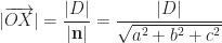
Given the equation of a plane: ax+by+cz=D, or in vector notation $\mathbf{r}\cdot \left( \begin{array}{c} a\\ b\\ c\\ \end{array}\right)=D$ , how do we find the (shortest) distance of a plane to the origin?

(When a question asks for the distance of a plane to the origin, by definition it means the shortest distance.)

One way to derive the formula is this:

Derivation

Let X be the point on the plane nearest to the origin.

$\overrightarrow{OX}$ must be perpendicular to the plane, i.e. parallel to the normal vector $\mathbf{n}=\left(\begin{array}{c}a\\b\\c\\\end{array}\right)$ .

Furthermore, X lies on the plane, hence we have $\boxed{\overrightarrow{OX}\cdot\mathbf{n}=D}$

Using the formula for dot product, we can get $|\overrightarrow{OX}\cdot\mathbf{n}|=|\overrightarrow{OX}||\mathbf{n}|\cos \theta=D$

Since $\overrightarrow{OX}$ is parallel to $\mathbf{n}$ , $\theta$ is either 0 or 180 degrees, hence $\cos \theta$ is either 1 or -1.

Thus, we have $|\overrightarrow{OX}||\mathbf{n}|=|D|$ .

The shortest distance from the point X to the origin is then $\displaystyle|\overrightarrow{OX}|=\frac{|D|}{|\mathbf{n}|}=\frac{|D|}{\sqrt{a^2+b^2+c^2}}$

Ans: Shortest distance from point to plane is $\displaystyle\boxed{\frac{|D|}{\sqrt{a^2+b^2+c^2}}}$

H2 Maths Condensed Notes and Prelim Papers

If you are looking for a short summarized H2 Maths Notes, with Prelim Papers to practice, do check out our Highly Condensed H2 Maths Notes!

Xinmin Secondary 2010 Prelim Paper I Q24 Solution (Challenging/Difficult Probability O Level Question)

Just to reblog this earlier post on a really challenging Probability O Level Question.

Also, do check out my other related posts on Probability:

Coursera Exciting New Probability Course

List of really useful Probability Formulae

Probability is becoming a really important branch of mathematics. One of the most famous Singaporean mathematicians is Professor Louis Chen Hsiao Yun who has a theorem named after him! (Stein-Chen method of Poisson approximation) Professor Chen researches on Probability.

To begin your journey in Probabilty, Introduction to Probability, 2nd Edition is a good book to start learning from. An intuitive, yet precise introduction to probability theory, stochastic processes, and probabilistic models used in science, engineering, economics, and related fields. You may also wish to refer to our comprehensive list of Recommended Undergraduate Books.

(One of the best books to begin your journey in studying the mysterious topic of Probability)

Mathtuition88

A bag A contains 9 black balls, 6 white balls and 3 red balls. A bag B contains 6 black balls, 2 white balls and 4 green balls. Ali takes out 1 ball from each bag randomly. When Ali takes out 1 ball from one bag, he will put it into the other bag and then takes out one ball from that bag. Find the probability that

(a) the ball is black from bag A, followed by white from bag B,
(b) both the balls are white in colour,
(c) the ball is black or white from bag B, followed by red from bag A,
(d) both the balls are of different colours,
(e) both the balls are not black or white in colours.

Solution:

(a) $latex displaystylefrac{9}{18}timesfrac{2}{13}=frac{1}{13}$

(b) Probability of white ball from bag A, followed by white ball from bag B=$latex displaystyle=frac{1}{2}timesfrac{6}{18}timesfrac{3}{13}=frac{1}{26}$

Probability of white from B, followed…

View original post 105 more words

Math and Motivation

Like many human endeavors, Math is one subject that requires motivation to excel.

There is this inspirational story that I found on https://schoolbag.sg/story/from-rock-bottom-to-top-of-the-class

With no interest in studying and thoroughly convinced he will never do well, M Thirukkumaran was on a downward spiral in secondary school and was almost retained in Secondary One and Two.

Fast forward nearly 10 years, Thiru, 23, is now studying Business Analytics at the National University of Singapore (NUS) under NEA and PUB’s National Environment and Water (NEW) Scholarship.

What turned Thiru a full 180 degrees around? It was the first taste of success, through the efforts of a teacher, Mr Tan Thiam Boon.

In Secondary Three at Monfort Secondary School, Thiru felt that he had hit rock bottom. During a rudimentary algebra test, he scored one mark out of a total score of 50. Instead of shaking his head in disbelief and despair, his mathematics teacher, Mr Tan, went out of his way to coach Thiru after school. But his efforts were in vain.

“Mentally, I had already accepted that I would not be able to do it,” said Thiru.

Undeterred, Mr Tan encouraged Thiru to pay full attention for the next topic, Trigonometry. Dejected and with little left to lose, Thiru came early to sit at the front of the class and followed the lesson attentively. About a week later, Mr Tan distributed the results of a test starting from the lowest to the highest scorers.

Thiru recalled the incident with great clarity.

“Naturally, I had expected my name to be the first to be called. But it was not and I was afraid my paper was lost. But instead, it was the last name called! I still remember the smile on Mr Tan’s face, and the confusion on everyone else’s that day. I sat dumbfounded. Mr Tan had managed to do what nobody else had. In one fell swoop, he eliminated the negative labels that society and I had placed on myself, and reinstated my confidence. More importantly, he showed me that I was capable, that I wasn’t a “delinquent” or a failure. It was akin to recovering from blindness.”

That initial spark ignited a passion, drive and desire to test his potential and accomplish what he did not even dare to imagine before. Thiru topped his class in mathematics and did well at the N-level and O-level examinations. At Tampines Junior College, his teachers gave him the opportunity to take H2 physics and mathematics, even though he did not take the prescribed secondary school subjects. Thiru’s hard work and determination paid off, often in the top 5% of the cohort for the regular examinations, and emerging as one of the college’s top students at the A-level examinations.

As a tutor, I know this is not easy. I have coached students from Fail to A grade. However, 1/50 is a really bad fail, and to achieve A in a matter of months requires extreme effort short of a miracle. For Thiru to overcome his challenges and extremely weak Math foundation to achieve his amazing accomplishments, required a motivational figure in the form of his Math teacher.

Such motivational teachers are rare, and I am glad that Thiru has found his mentor.

Helen Exley — ‘Books can be dangerous. The best ones should be labeled This could change your life.’ Books are another source of motivation. For those who have not yet found their motivational figure, do not wait as true motivational teachers are few and far between. To encounter one like Thiru requires luck and good fortune. However, good motivational books are there and available if you look for it. I have compiled a list of Motivational Books for the Student, which is available by clicking on the link.

In Math, you must always believe that you can solve the answer, in order to solve it. Just like Thiru, if you believe in yourself, you can do it! A nice book to read about Math and Motivation is Math Doesn’t Suck: How to Survive Middle School Math Without Losing Your Mind or Breaking a Nail. Ideal for teenagers, this book features an award winning actress who struggled with math, but later overcame her fears to be one of the top in UCLA Math faculty. Even Terence Tao praised her.

Poll: Is Math easier or more difficult than other subjects?

Hi everyone, please vote on this poll, and forward it to your friends! You may click on the buttons below this post to post to Facebook or Twitter!

Recently, I was reading this article online (Science and maths exams are harder than arts subjects, say researchers) by a reputed online magazine Guardian. In it, Durham researchers have found that, “At A-level, science, maths and technology subjects are not just more difficult than the non-sciences, they are without exception among the hardest of all A-levels. At GCSE, the sciences are a little more difficult than the non-sciences.“.

However, there are many rebuttals, for instance: Ian McNeilly, director of the National Association for the Teaching of English, said: “It seems scientists, on the one hand, decry the quality of their intake at universities and, on the other, say that their exams are so very hard. Any view of English as a ‘soft option’ is absolute nonsense. If the scientists tried to do it, they would find it wasn’t such a breeze.”

My view is that on one hand, yes Math is hard especially if the student doesn’t know what he/she is doing. It is very possible to get zero marks if the student makes a careless mistake in the very first step, or goes completely off tangent in approaching the question. However, in humanities, the only possible way to get zero marks is to hand up a blank script of paper. As long as you write something, most likely you will get some marks.

However, if the student knows what he/she is doing, and has sufficient practice, Math is actually easier. (We are not talking about the Riemann Hypothesis here, just high school and perhaps up to college mathematics.) In Math, we often hear of students scoring full marks, which they fully deserve if they know how to do every question. On the other hand, it is impossible to score full marks in English Literature, especially if there is an essay component. No essay is perfect!

Of course, there are ways to be good at both the Science and the Arts. For instance, From STEM to STEAM: Using Brain-Compatible Strategies to Integrate the Arts is a highly regarded book on how to integrate arts curriculum into STEM (Science, Tech, Engineering, Mathematics) courses.

Personally, I will not dismiss arts as “easy”, as arts do need time and effort to achieve mastery. Not everyone can write essays like Shakespeare, nor can everyone write calligraphy like the famous Wang Xizhi of China.

However, in the context of examinations, based on my personal experience, and readings on the internet, Math / Hard Science exams are indeed harder and more difficult than arts exams. This has a very negative effect of students dropping Math / Science subjects to major in “easier” subjects. Another point of concern is grade inflation in other subjects.

Most importantly, what do you think? Is Math easier or harder than other subjects?

Please vote, and forward this to your friends for voting! I will be really interested to know the results.

Latest Updates on Mathtuition88.blogspot.com

Just to update on the latest blog posts at http://mathtuition88.blogspot.com. I am trying to bring up the page rank for my Blogspot site, hence blogging there for the time being.

Topics taught in JC 1 / JC 2 H2 Maths Many schools are now functioning more or less independently, and as a result teach various JC topics in different orders. Here is a suggested order followed by HCI, and to some extent RJC.
H2 Maths Syllabus and Formula Sheet can be found here.
Some amazing statistics about the top scorers of the IB program. Did you know the tiny Singapore island with only a few schools (notably ACS(I) and SJI) taking the IB syllabus actually produces more top scorers than the entire Australian continent? Asia power?
Noah Ark is round or square? Check out this link which debates whether the Noah’s Ark is round or square, based on mathematics.
O Level Top Scorer 2015
Winnie The Pooh Maths Olympiad question
The latest trend: Parents going for Maths Tuition

This book Why Before How: Singapore Math Computation Strategies, Grades 1-6 is surprisingly very popular. As an Amazon Affiliate, one of the most popular book I promote on my site is actually this book. It is a Singapore Math book that focuses on the “Why” before the “How”, which is very important as nowadays questions are designed to be solved using thinking, not just mechanical procedures.

Math of QZ8501 (Sum of 3 numbers that add up to 8888)

Source: http://mathtuition88.blogspot.sg/2014/12/math-of-qz8501-sum-of-3-numbers-that.html

We sincerely hope that Captain Iriyanto, the pilot of missing AirAsia flight QZ8501, and all other passengers survive and return safely. Hopefully the plane will be found soon.

Something mysterious about the recent missing airplanes is that their numbers add up to 8888, a mystical number in Chinese culture. MH17, MH370, QZ8501, 17+370+8501=8888.

We have calculated that it is not a common event at all, it is rarer than winning the top prize in 4D, a lottery in Singapore.

Probability of 3 random numbers (from 1 to 9999) adding to 8888: 0.0039497% , or around 1 in 25,000.

Probability of winning the First Prize in 4D: 0.01%, or 1 in 10,000.

Featured Book:

Introduction to Probability, 2nd Edition

An intuitive, yet precise introduction to probability theory, stochastic processes, and probabilistic models used in science, engineering, economics, and related fields. The 2nd edition is a substantial revision of the 1st edition, involving a reorganization of old material and the addition of new material. The length of the book has increased by about 25 percent. The main new feature of the 2nd edition is thorough introduction to Bayesian and classical statistics.

Star Wars Math

With the Star Wars Episode 7 coming up, all Star Wars fans are really excited. The trailer alone has reached 50 million views, barely a month after it was released.

$math of star wars$ Wait, can Star Wars be related to Math? Yes it can! Check out The Math of Star Wars which describes a Math related question related to Star Wars! As a Math Tutor, I try my best to relate anything and everything to Math! 😛

Christmas is ending soon, and hope everyone had a nice day, and happy new Year!

Featured Book:

Star Wars Workbook: 1st Grade Math

Does your child love Star Wars but hate math? Well, this might just work! A highly rated Workbook based on Star Wars.

Math Formula in WordPress vs Blogspot

Refering to How to write Math Formulas on Blogspot / Blogger, Blogspot is also capable of rendering beautiful Math Equations based on LaTeX.

blogger latex — Produced by Blogspot using MathJax

Blogger uses MathJax for rendering the Math Formulas, which look like the ones shown above.

Let’s try the WordPress version and readers can judge for themselves which is better.

$\displaystyle a^p \equiv a \pmod p$

$\displaystyle\int_0^{\frac{\pi}{2}} \sin x\ dx=1$

My personal opinion is: they look the same to be honest. However, the Blogger way of typing is much more convenient, just using $ and $$, as opposed to WordPress requiring “$latex” and “$latex\displaystyle”, which is more cumbersome especially for long texts. However, experts like Terence Tao have opted for WordPress, which shows that WordPress does probably have some advantages.

Featured Book:

The LaTeX Companion (Tools and Techniques for Computer Typesetting)