
This is a very nice and concise 8 minute introduction to cohomology. Very clear and tells you the gist of cohomology.
Tag: Topology
Recommended Books for Spectral Sequences
Best Spectral Sequence Book
So far the most comprehensive book looks like McCleary’s book: A User’s Guide to Spectral Sequences. It is also suitable for those interested in the algebraic viewpoint. W.S. Massey wrote a very positive review to this book.
A User’s Guide to Spectral Sequences (Cambridge Studies in Advanced Mathematics)

Another book is Rotman’s An Introduction to Homological Algebra (Universitext). This book is from a homological algebra viewpoint. Rotman has a nice easy-going style, that made his books very popular to read.
The classic book may be MacLane’s Homology (Classics in Mathematics). This may be harder to read (though to be honest all books on spectral sequences are hard).
***Update: I found another book that gives a very nice presentation of certain spectral sequences, for instance the Bockstein spectral sequence. The book is Algebraic Methods in Unstable Homotopy Theory (New Mathematical Monographs) by Joseph Neisendorfer.

Topology application to Physics
Source: https://www.scientificamerican.com/article/the-strange-topology-that-is-reshaping-physics/?W
The Strange Topology That Is Reshaping Physics
Topological effects might be hiding inside perfectly ordinary materials, waiting to reveal bizarre new particles or bolster quantum computing
Charles Kane never thought he would be cavorting with topologists. “I don’t think like a mathematician,” admits Kane, a theoretical physicist who has tended to focus on tangible problems about solid materials. He is not alone. Physicists have typically paid little attention to topology—the mathematical study of shapes and their arrangement in space. But now Kane and other physicists are flocking to the field.
In the past decade, they have found that topology provides unique insight into the physics of materials, such as how some insulators can sneakily conduct electricity along a single-atom layer on their surfaces.
Some of these topological effects were uncovered in the 1980s, but only in the past few years have researchers begun to realize that they could be much more prevalent and bizarre than anyone expected. Topological materials have been “sitting in plain sight, and people didn’t think to look for them”, says Kane, who is at the University of Pennsylvania in Philadelphia.
Now, topological physics is truly exploding: it seems increasingly rare to see a paper on solid-state physics that doesn’t have the word topology in the title. And experimentalists are about to get even busier. A study on page 298 of this week’s Nature unveils an atlas of materials that might host topological effects, giving physicists many more places to go looking for bizarre states of matter such as Weyl fermions or quantum-spin liquids.
Read more at: https://www.scientificamerican.com/article/the-strange-topology-that-is-reshaping-physics/?WT.mc_id=SA_WR_20170726
Summary: Shapes, radius functions and persistent homology
This is a summary of a talk by Professor Herbert Edelsbrunner, IST Austria. The PDF slides can be found here: persistent homology slides.
Biogeometry (2:51 in video)
We can think of proteins as a geometric object by replacing every atom by a sphere (possibly different radii). Protein is viewed as union of balls in 
Decompose into Voronoi domains 
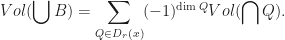
Inclusion-Exclusion Theorem:
Volume of protein 

Nerve Theorem: Union of sets have same homotopy type as nerve (stronger than having isomorphic homology groups).
Wrap (14:04 in video)
Collapses: 01 collapse means 0 dimensional and 1 dimensional simplices disappear (something like deformation retract).
Interval: Simplices that are removed in a collapse (always a skeleton of a cube in appropriate dimension)
Generalised Discrete Morse Function (Forman 1998): Generalised discrete vector field 
Critical simplex: The only simplex in an interval (when a critical simplex is added, the homotopy type changes)
Lower set of critical simplex: all the nodes that lead up to the critical simplex.
Wrap complex is the union of lower sets.
Persistence (38:00 in video)
Betti numbers in 


Incremental Algorithm to compute Betti numbers (40:50 in video). [Deffimado, E., 1995]. Every time a simplex is added, either a Betti number goes up (birth) or goes down (death).

Stability of persistence: small change in position of points leads to similar persistence diagram.
Bottleneck distance between two diagrams is length of longest edge in minimizing matching. Theorem: 
Expectation (51:30 in video)
Poisson point process: Like uniform distribution but over entire space. Number of points in region is proportional to size of region. Proportionality constant is density 
Paper: Expectations in 
Reduces to question (Three points in circle): Given three points in a circle, what is the probability that the triangle (with the 3 points as vertices) contains the center of the circle? Ans: 1/4 [Wendel 1963].
Brain has 11 dimensions
One of the possible applications of algebraic topology is in studying the brain, which is known to be very complicated.
Site: https://www.wired.com/story/the-mind-boggling-math-that-maybe-mapped-the-brain-in-11-dimensions/
If you can call understanding the dynamics of a virtual rat brain a real-world problem. In a multimillion-dollar supercomputer in a building on the same campus where Hess has spent 25 years stretching and shrinking geometric objects in her mind, lives one of the most detailed digital reconstructions of brain tissue ever built. Representing 55 distinct types of neurons and 36 million synapses all firing in a space the size of pinhead, the simulation is the brainchild of Henry Markram.
Markram and Hess met through a mutual researcher friend 12 years ago, right around the time Markram was launching Blue Brain—the Swiss institute’s ambitious bid to build a complete, simulated brain, starting with the rat. Over the next decade, as Markram began feeding terabytes of data into an IBM supercomputer and reconstructing a collection of neurons in the sensory cortex, he and Hess continued to meet and discuss how they might use her specialized knowledge to understand what he was creating. “It became clearer and clearer algebraic topology could help you see things you just can’t see with flat mathematics,” says Markram. But Hess didn’t officially join the project until 2015, when it met (and some would say failed) its first big public test.
In October of that year, Markram led an international team of neuroscientists in unveiling the first Blue Brain results: a simulation of 31,000 connected rat neurons that responded with waves of coordinated electricity in response to an artificial stimulus. The long awaited, 36-page paper published in Cell was not greeted as the unequivocal success Markram expected. Instead, it further polarized a research community already divided by the audacity of his prophesizing and the insane amount of money behind the project.
Two years before, the European Union had awarded Markram $1.3 billion to spend the next decade building a computerized human brain. But not long after, hundreds of EU scientists revolted against that initiative, the Human Brain Project. In the summer of 2015, they penned an open letter questioning the scientific value of the project and threatening to boycott unless it was reformed. Two independent reviews agreed with the critics, and the Human Brain Project downgraded Markram’s involvement. It was into this turbulent atmosphere that Blue Brain announced its modest progress on its bit of simulated rat cortex.
Read more at the link above.
Guide to Starting Javaplex (With Matlab)
Guide to Starting Javaplex (With Matlab)
Step 1)
Visit https://appliedtopology.github.io/javaplex/ and download the Persistent Homology and Topological Data Analysis Library
2)
Download the tutorial at http://www.math.colostate.edu/~adams/research/javaplex_tutorial.pdf and jump to section 1.3. Installation for Matlab.
3)
In Matlab, change Matlab’s “Current Folder” to the directory matlab examples that you just extracted from the zip file.
(See https://www.mathworks.com/help/matlab/ref/cd.html to change current folder)
Type this in Matlab: cd /…/matlab_examples
Where … depends on where you put the folder
4) In the tutorial (from the link given in step 2), proceed to follow the instructions starting from “In Matlab, change Matlab’s “Current Folder” to the directory matlab examples that you just extracted from the zip file. In the Matlab command window, run the load javaplex.m file.”.
5) Test: Run example 3.2 (House example) by typing in the code (following the tutorial)

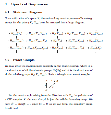
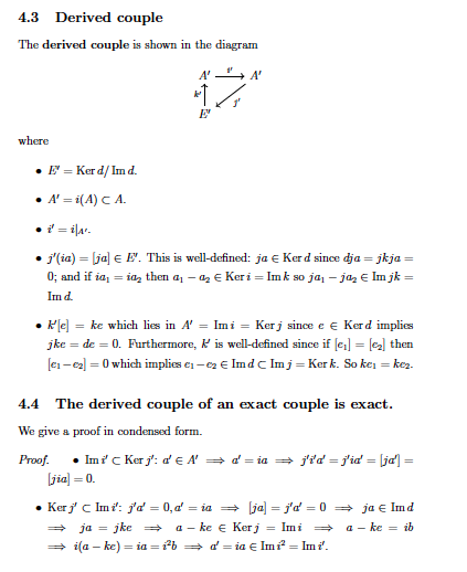
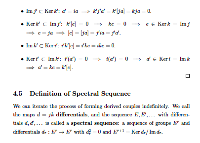
How the Staircase Diagram changes when we pass to derived couple (Spectral Sequence)
Set 


When we pass to the derived couple, each group 
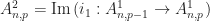


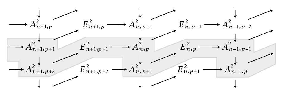
The maps 
![j_2(i_1a)=[j_1a]](https://s0.wp.com/latex.php?latex=j_2%28i_1a%29%3D%5Bj_1a%5D&bg=ffffff&fg=1a1a1a&s=0&c=20201002)


Relative Homology Groups
Given a space 


We have a chain complex 


Relative cycles
Elements of 


Relative boundary
A relative cycle 


Long Exact Sequence (Relative Homology)
There is a long exact sequence of homology groups:

The boundary map 
![[\alpha]\in H_n(X,A)](https://s0.wp.com/latex.php?latex=%5B%5Calpha%5D%5Cin+H_n%28X%2CA%29&bg=ffffff&fg=1a1a1a&s=0&c=20201002)
![\partial[\alpha]](https://s0.wp.com/latex.php?latex=%5Cpartial%5B%5Calpha%5D&bg=ffffff&fg=1a1a1a&s=0&c=20201002)


Exact sequence (Quotient space)
Exact sequence (Quotient space)
If 
where 


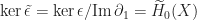
Reduced homology of spheres (Proof)


For 


Exactness of the sequence then implies that the maps 


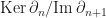
Reduced Homology
Define the reduced homology groups 


Relation between 
Since 


Klein Bottle as Gluing of Two Mobius Bands

This is a nice picture on how the Klein bottle can be formed by gluing two Mobius bands together. Very neat and self-explanatory!
Source: https://math.stackexchange.com/questions/907176/klein-bottle-as-two-m%C3%B6bius-strips
Mayer-Vietoris Sequence applied to Spheres
Mayer-Vietoris Sequence
For a pair of subspaces 
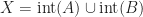
Example:
Let 


We obtain isomorphisms 

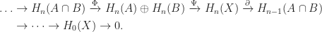
Spectral Sequence
Spectral Sequence is one of the advanced tools in Algebraic Topology. The following definition is from Hatcher’s 5th chapter on Spectral Sequences. The staircase diagram looks particularly impressive and intimidating at the same time.
Unfortunately, my LaTeX to WordPress Converter app can’t handle commutative diagrams well, so I will upload a printscreen instead.
Echelon Form Lemma (Column Echelon vs Smith Normal Form)
The pivots in column-echelon form are the same as the diagonal elements in (Smith) normal form. Moreover, the degree of the basis elements on pivot rows is the same in both forms.
Proof:
Due to the initial sort, the degree of row basis elements 


We may then eliminate non-zero elements below pivots using row operations that do not change the pivot elements or the degrees of the row basis elements. Finally, we place the matrix in (Smith) normal form with row and column swaps.
Persistent Homology Algorithm
Algorithm for Fields
In this section we describe an algorithm for computing persistent homology over a field.
We use the small filtration as an example and compute over 
A filtered simplicial complex with new simplices added at each stage. The integers on the bottom row corresponds to the degrees of the simplices of the filtration as homogenous elements of the persistence module.
The persistence module corresponds to a ![\mathbb{Z}_2[t]](https://s0.wp.com/latex.php?latex=%5Cmathbb%7BZ%7D_2%5Bt%5D&bg=ffffff&fg=1a1a1a&s=0&c=20201002)


We have 

![\displaystyle M_1=\begin{bmatrix}[c|ccccc] &ab &bc &cd &ad &ac\\ \hline d & 0 & 0 & t & t & 0\\ c & 0 & 1 & t & 0 & t^2\\ b & t & t & 0 & 0 & 0\\ a &t &0 &0 &t^2 &t^3 \end{bmatrix}.](https://s0.wp.com/latex.php?latex=%5Cdisplaystyle+M_1%3D%5Cbegin%7Bbmatrix%7D%5Bc%7Cccccc%5D++%26ab+%26bc+%26cd+%26ad+%26ac%5C%5C+%5Chline++d+%26+0+%26+0+%26+t+%26+t+%26+0%5C%5C++c+%26+0+%26+1+%26+t+%26+0+%26+t%5E2%5C%5C++b+%26+t+%26+t+%26+0+%26+0+%26+0%5C%5C++a+%26t+%260+%260+%26t%5E2+%26t%5E3++%5Cend%7Bbmatrix%7D.&bg=ffffff&fg=1a1a1a&s=0&c=20201002)
In general, any representation 


We need to represent 

We compute the representations inductively in dimension. Since 


For the inductive step, we need to compute a homogeneous basis for 


Source: “Computing Persistent Homology” by Zomorodian & Carlsson
De Rham Cohomology
De Rham Cohomology is a very cool sounding term in advanced math. This blog post is a short introduction on how it is defined.
Also, do check out our presentation on the relation between De Rham Cohomology and physics: De Rham Cohomology.
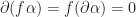
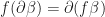
Definition:
A differential form 


Corollary:
Since 
Definition:
Let 

Let 
Since every exact form is closed, hence 
The de Rham cohomology of

The quotient vector space construction induces an equivalence relation on


The equivalence class of a closed form ![[\omega]](https://s0.wp.com/latex.php?latex=%5B%5Comega%5D&bg=ffffff&fg=1a1a1a&s=0&c=20201002)
Singular Homology
A singular 


![\displaystyle \partial_n(\sigma)=\sum_i(-1)^i\sigma|[v_0,\dots,\widehat{v_i},\dots,v_n].](https://s0.wp.com/latex.php?latex=%5Cdisplaystyle+%5Cpartial_n%28%5Csigma%29%3D%5Csum_i%28-1%29%5Ei%5Csigma%7C%5Bv_0%2C%5Cdots%2C%5Cwidehat%7Bv_i%7D%2C%5Cdots%2Cv_n%5D.&bg=ffffff&fg=1a1a1a&s=0&c=20201002)
The singular homology group is defined as 
Mapping Cone Theorem
Mapping cone
Let 


![[1,x]\in CX](https://s0.wp.com/latex.php?latex=%5B1%2Cx%5D%5Cin+CX&bg=ffffff&fg=1a1a1a&s=0&c=20201002)


Proposition:
For any map 


Proof:
By an earlier proposition (2.32 in \cite{Switzer2002}), 

(

![\tilde{h}(y_0,[t,x])=\psi[t,x]](https://s0.wp.com/latex.php?latex=%5Ctilde%7Bh%7D%28y_0%2C%5Bt%2Cx%5D%29%3D%5Cpsi%5Bt%2Cx%5D&bg=ffffff&fg=1a1a1a&s=0&c=20201002)
![\tilde{h}(y,[0,x])=g(y)](https://s0.wp.com/latex.php?latex=%5Ctilde%7Bh%7D%28y%2C%5B0%2Cx%5D%29%3Dg%28y%29&bg=ffffff&fg=1a1a1a&s=0&c=20201002)
![\tilde{h}(y_0,[0,x])=\psi[0,x]=g(y_0)=z_0](https://s0.wp.com/latex.php?latex=%5Ctilde%7Bh%7D%28y_0%2C%5B0%2Cx%5D%29%3D%5Cpsi%5B0%2Cx%5D%3Dg%28y_0%29%3Dz_0&bg=ffffff&fg=1a1a1a&s=0&c=20201002)
![\displaystyle \tilde{h}(y_0,[1,x])=\psi[1,x]=gf(x)=\tilde{h}(f(x),[0,x]),](https://s0.wp.com/latex.php?latex=%5Cdisplaystyle+%5Ctilde%7Bh%7D%28y_0%2C%5B1%2Cx%5D%29%3D%5Cpsi%5B1%2Cx%5D%3Dgf%28x%29%3D%5Ctilde%7Bh%7D%28f%28x%29%2C%5B0%2Cx%5D%29%2C&bg=ffffff&fg=1a1a1a&s=0&c=20201002)


![h[y,[0,x]]=\tilde{h}(y,[0,x])=g(y)](https://s0.wp.com/latex.php?latex=h%5By%2C%5B0%2Cx%5D%5D%3D%5Ctilde%7Bh%7D%28y%2C%5B0%2Cx%5D%29%3Dg%28y%29&bg=ffffff&fg=1a1a1a&s=0&c=20201002)

(

![\psi([t,x])=h[y_0,[t,x]]](https://s0.wp.com/latex.php?latex=%5Cpsi%28%5Bt%2Cx%5D%29%3Dh%5By_0%2C%5Bt%2Cx%5D%5D&bg=ffffff&fg=1a1a1a&s=0&c=20201002)
![\psi([0,x])=h[y_0,[0,x]]=z_0](https://s0.wp.com/latex.php?latex=%5Cpsi%28%5B0%2Cx%5D%29%3Dh%5By_0%2C%5B0%2Cx%5D%5D%3Dz_0&bg=ffffff&fg=1a1a1a&s=0&c=20201002)
![\displaystyle \psi([1,x])=h[y_0,[1,x]]=h[f(x),[0,x]]=gf(x).](https://s0.wp.com/latex.php?latex=%5Cdisplaystyle+%5Cpsi%28%5B1%2Cx%5D%29%3Dh%5By_0%2C%5B1%2Cx%5D%5D%3Dh%5Bf%28x%29%2C%5B0%2Cx%5D%5D%3Dgf%28x%29.&bg=ffffff&fg=1a1a1a&s=0&c=20201002)

Tangent space (Derivation definition)
Let 

The tangent space to 


Homology Group of some Common Spaces
Homology of Circle

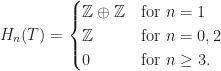
Homology of Torus
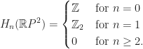
Homology of Real Projective Plane
Homology of Klein Bottle

Summary of Persistent Homology
We summarize the work so far and relate it to previous results. Our input is a filtered complex 


We need to choose compatible bases across the filtration (compatible bases for 


Specifically, each 


A natural question is to ask when 


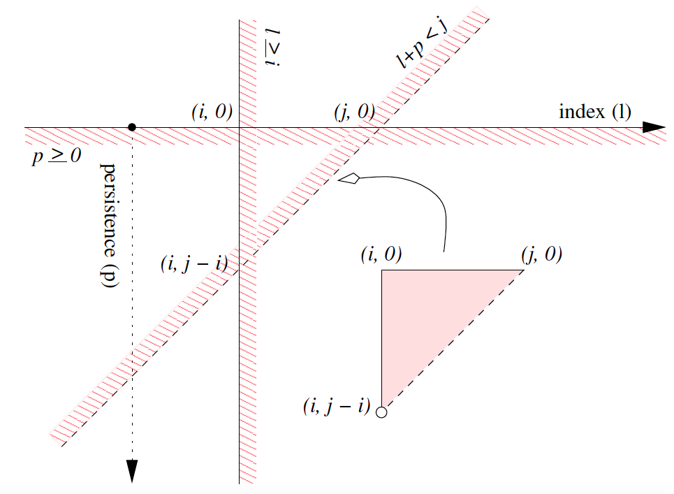
The triangular region gives us the values for which the
Let 


Hence, computing persistent homology over a field is equivalent to finding the corresponding set of
Source: “Computing Persistent Homology” by Zomorodian and Carlsson
Structure Theorem for finitely generated (graded) modules over a PID
If 

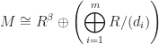


Similarly, every graded module 


Persistence Interval
Next, we want to parametrize the isomorphism classes of the ![F[t]](https://s0.wp.com/latex.php?latex=F%5Bt%5D&bg=ffffff&fg=1a1a1a&s=0&c=20201002)
A 
We may associate a graded 
![\displaystyle Q(i,j)=\Sigma^i F[t]/(t^{j-i})](https://s0.wp.com/latex.php?latex=%5Cdisplaystyle+Q%28i%2Cj%29%3D%5CSigma%5Ei+F%5Bt%5D%2F%28t%5E%7Bj-i%7D%29&bg=ffffff&fg=1a1a1a&s=0&c=20201002)

![Q(i,+\infty)=\Sigma^iF[t]](https://s0.wp.com/latex.php?latex=Q%28i%2C%2B%5Cinfty%29%3D%5CSigma%5EiF%5Bt%5D&bg=ffffff&fg=1a1a1a&s=0&c=20201002)
For a set of 

We may now restate the correspondence as follows.
The correspondence 
Hence, the isomorphism classes of persistence modules of finite type over
Homogenous / Graded Ideal
Let 


An ideal in a graded ring is homogenous if and only if it is a graded submodule. The intersections of a homogenous ideal 

Persistence module and Graded Module
We show that the persistent homology of a filtered simplicial complex is the standard homology of a particular graded module over a polynomial ring.
First we review some definitions.
A graded ring is a ring 


A graded ring 


Polynomial ring with standard grading:
We may grade the polynomial ring ![R[t]](https://s0.wp.com/latex.php?latex=R%5Bt%5D&bg=ffffff&fg=1a1a1a&s=0&c=20201002)


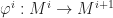
Graded module:
A graded module is a left module 

Let 
We now equip 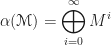


The action of 
That is,

Source: “Computing Persistent Homology” by Zomorodian and Carlsson.
Persistence module and Finite type
A persistence module 

For example, the homology of a persistence complex is a persistence module, where 
A persistence complex 


If 

Homotopy for Maps vs Paths
Homotopy (of maps)
A homotopy is a family of maps 


Homotopy of paths
A homotopy of paths in a space 

(i) The endpoints 

(ii) The associated map 

When two paths 

The above two definitions are related, since a path is a special kind of map 
Universal Property of Quotient Groups (Hungerford)
If 


This can be used to prove the following proposition:
A chain map 


Proof:
The relation 


For 

Some Homology Definitions
Chain Complex
A sequence of homomorphisms of abelian groups 


Elements of 

Introduction to Persistent Homology (Cech and Vietoris-Rips complex)
Motivation
Data is commonly represented as an unordered sequence of points in the Euclidean space
For data points in 
From point cloud data to simplicial complexes
To convert a collection of points 
Given a set of points 


Given a set of points 

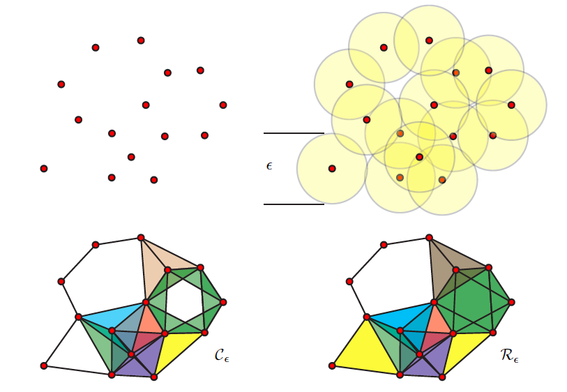
Top left: A fixed set of points. Top right: Closed balls of radius 

Natural Equivalence relating Suspension and Loop Space
Theorem:
If 


![\displaystyle A: [Z\wedge X, *; Y,y_0]\to [X, x_0; (Y,y_0)^{(Z,z_0)}, f_0]](https://s0.wp.com/latex.php?latex=%5Cdisplaystyle+A%3A+%5BZ%5Cwedge+X%2C+%2A%3B+Y%2Cy_0%5D%5Cto+%5BX%2C+x_0%3B+%28Y%2Cy_0%29%5E%7B%28Z%2Cz_0%29%7D%2C+f_0%5D&bg=ffffff&fg=1a1a1a&s=0&c=20201002)
![A[f]=[\hat{f}]](https://s0.wp.com/latex.php?latex=A%5Bf%5D%3D%5B%5Chat%7Bf%7D%5D&bg=ffffff&fg=1a1a1a&s=0&c=20201002)


![(\hat{f}(x))(z)=f[z,x]](https://s0.wp.com/latex.php?latex=%28%5Chat%7Bf%7D%28x%29%29%28z%29%3Df%5Bz%2Cx%5D&bg=ffffff&fg=1a1a1a&s=0&c=20201002)
We need the following two propositions in order to prove the theorem.
Proposition
\label{prop13}
The exponential function 

Proposition
\label{prop8}
If 


Proof of Theorem
i) 


![f[z,x]=\bar{f}(z,x)=(f'(x))(z)](https://s0.wp.com/latex.php?latex=f%5Bz%2Cx%5D%3D%5Cbar%7Bf%7D%28z%2Cx%29%3D%28f%27%28x%29%29%28z%29&bg=ffffff&fg=1a1a1a&s=0&c=20201002)

![A[f]=[f']](https://s0.wp.com/latex.php?latex=A%5Bf%5D%3D%5Bf%27%5D&bg=ffffff&fg=1a1a1a&s=0&c=20201002)
ii) 
![A[f]=A[g]](https://s0.wp.com/latex.php?latex=A%5Bf%5D%3DA%5Bg%5D&bg=ffffff&fg=1a1a1a&s=0&c=20201002)


![H([z,x],t)=\bar{H}(z,x,t)=(H'(x,t))(z)](https://s0.wp.com/latex.php?latex=H%28%5Bz%2Cx%5D%2Ct%29%3D%5Cbar%7BH%7D%28z%2Cx%2Ct%29%3D%28H%27%28x%2Ct%29%29%28z%29&bg=ffffff&fg=1a1a1a&s=0&c=20201002)
![H_0([z,x])=(H_0'(x))(z)=(\hat{f}(x))(z)=f[z,x]](https://s0.wp.com/latex.php?latex=H_0%28%5Bz%2Cx%5D%29%3D%28H_0%27%28x%29%29%28z%29%3D%28%5Chat%7Bf%7D%28x%29%29%28z%29%3Df%5Bz%2Cx%5D&bg=ffffff&fg=1a1a1a&s=0&c=20201002)
![H_1([z,x])=(H_1'(x))(z)=(\hat{g}(x))(z)=g[z,x]](https://s0.wp.com/latex.php?latex=H_1%28%5Bz%2Cx%5D%29%3D%28H_1%27%28x%29%29%28z%29%3D%28%5Chat%7Bg%7D%28x%29%29%28z%29%3Dg%5Bz%2Cx%5D&bg=ffffff&fg=1a1a1a&s=0&c=20201002)
![[f]=[g]](https://s0.wp.com/latex.php?latex=%5Bf%5D%3D%5Bg%5D&bg=ffffff&fg=1a1a1a&s=0&c=20201002)

Loop space
If 


Suspension
If 


Corollary (Natural Equivalence relating 

If
![\displaystyle A: [SX, *; Y,y_0]\to [X, x_0; \Omega Y, \omega_0].](https://s0.wp.com/latex.php?latex=%5Cdisplaystyle+A%3A+%5BSX%2C+%2A%3B+Y%2Cy_0%5D%5Cto+%5BX%2C+x_0%3B+%5COmega+Y%2C+%5Comega_0%5D.&bg=ffffff&fg=1a1a1a&s=0&c=20201002)
Fundamental Group of S^n is trivial if n>=2

We need the following lemma:
If a space 


Proof:
Take 


Choose a basepoint 


Functors, Homotopy Sets and Groups
Functors
Definition:
A functor 
– For each object 

– For each 

Furthermore,
– For each object 

– For 


Definition:
A cofunctor (also called contravariant functor) 
– For each object 
– For each 
– For each object 
– For each 
Example
Given a fixed pointed space 

![F_K(X,x_0)=[K,k_0; X,x_0]\in\mathscr{PS}](https://s0.wp.com/latex.php?latex=F_K%28X%2Cx_0%29%3D%5BK%2Ck_0%3B+X%2Cx_0%5D%5Cin%5Cmathscr%7BPS%7D&bg=ffffff&fg=1a1a1a&s=0&c=20201002)


![F_K(f)\in\hom([K,k_0; X,x_0],[K,k_0;Y,y_0])](https://s0.wp.com/latex.php?latex=F_K%28f%29%5Cin%5Chom%28%5BK%2Ck_0%3B+X%2Cx_0%5D%2C%5BK%2Ck_0%3BY%2Cy_0%5D%29&bg=ffffff&fg=1a1a1a&s=0&c=20201002)
![\displaystyle F_k(f)[g]=[f\circ g]\in[K,k_0; Y,y_0]](https://s0.wp.com/latex.php?latex=%5Cdisplaystyle+F_k%28f%29%5Bg%5D%3D%5Bf%5Ccirc+g%5D%5Cin%5BK%2Ck_0%3B+Y%2Cy_0%5D&bg=ffffff&fg=1a1a1a&s=0&c=20201002)
![[g]\in [K,k_0; X,x_0]](https://s0.wp.com/latex.php?latex=%5Bg%5D%5Cin+%5BK%2Ck_0%3B+X%2Cx_0%5D&bg=ffffff&fg=1a1a1a&s=0&c=20201002)
We can check the two axioms:
– ![F_k(1_X)[g]=[1_X\circ g]=[g]](https://s0.wp.com/latex.php?latex=F_k%281_X%29%5Bg%5D%3D%5B1_X%5Ccirc+g%5D%3D%5Bg%5D&bg=ffffff&fg=1a1a1a&s=0&c=20201002)
![[g]\in[K,k_0; X, x_0]](https://s0.wp.com/latex.php?latex=%5Bg%5D%5Cin%5BK%2Ck_0%3B+X%2C+x_0%5D&bg=ffffff&fg=1a1a1a&s=0&c=20201002)
– For 

![\displaystyle F_K(h\circ f)[g]=[h\circ f\circ g]=F_K(h)\circ F_K(f)[g]\in[K,k_0; Z,z_0]](https://s0.wp.com/latex.php?latex=%5Cdisplaystyle+F_K%28h%5Ccirc+f%29%5Bg%5D%3D%5Bh%5Ccirc+f%5Ccirc+g%5D%3DF_K%28h%29%5Ccirc+F_K%28f%29%5Bg%5D%5Cin%5BK%2Ck_0%3B+Z%2Cz_0%5D&bg=ffffff&fg=1a1a1a&s=0&c=20201002)
![[g]\in[K,k_0; X,x_0]](https://s0.wp.com/latex.php?latex=%5Bg%5D%5Cin%5BK%2Ck_0%3B+X%2Cx_0%5D&bg=ffffff&fg=1a1a1a&s=0&c=20201002)
Similarly, we can define a cofunctor 
![F_K^*(X,x_0)=[X,x_0; K,k_0]](https://s0.wp.com/latex.php?latex=F_K%5E%2A%28X%2Cx_0%29%3D%5BX%2Cx_0%3B+K%2Ck_0%5D&bg=ffffff&fg=1a1a1a&s=0&c=20201002)
![\displaystyle F_K(f)[g]=[g\circ f]\in[X,x_0; K,k_0]](https://s0.wp.com/latex.php?latex=%5Cdisplaystyle+F_K%28f%29%5Bg%5D%3D%5Bg%5Ccirc+f%5D%5Cin%5BX%2Cx_0%3B+K%2Ck_0%5D&bg=ffffff&fg=1a1a1a&s=0&c=20201002)
![[g]\in[Y,y_0; K,k_0]](https://s0.wp.com/latex.php?latex=%5Bg%5D%5Cin%5BY%2Cy_0%3B+K%2Ck_0%5D&bg=ffffff&fg=1a1a1a&s=0&c=20201002)
Note that if 


Homotopy Sets and Groups
Theorem:
If
We need the following two propositions in order to prove the theorem.
Proposition 1:
The exponential function
Proposition 2:
If
Algebraic Topology: Fundamental Group
Homotopy of paths
A homotopy of paths in a space
(i) The endpoints
(ii) The associated map
When two paths
Example: Linear Homotopies
Any two paths 

Simply-connected
A space is called simply-connected if it is path-connected and has trivial fundamental group.
A space
Path-connectedness is the existence of paths connecting every pair of points, so we need to be concerned only with the uniqueness of connecting paths.
(


(


A basic property of the product topology is that a map 


Hence a loop 


Similarly, a homotopy 

Thus we obtain a bijection 
![[f]\mapsto([g],[h])](https://s0.wp.com/latex.php?latex=%5Bf%5D%5Cmapsto%28%5Bg%5D%2C%5Bh%5D%29&bg=ffffff&fg=1a1a1a&s=0&c=20201002)
Note: The condition that 

Topological Monster: Alexander horned sphere
Very interesting object indeed. Also see this previous video on How to Unlock Interlocked Fingers Topologically?
The horned sphere, together with its inside, is a topological 3-ball, the Alexander horned ball, and so is simply connected; i.e., every loop can be shrunk to a point while staying inside. The exterior is not simply connected, unlike the exterior of the usual round sphere; a loop linking a torus in the above construction cannot be shrunk to a point without touching the horned sphere. (Wikipedia)
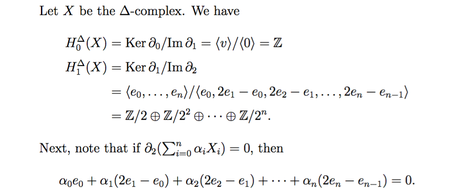
Hatcher 2.1.6

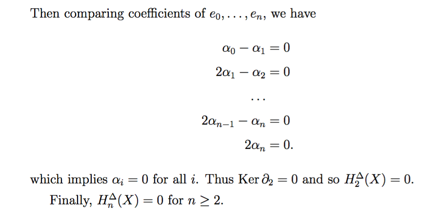
Compute the simplicial homology groups of the 


![[v_0,v_1]](https://s0.wp.com/latex.php?latex=%5Bv_0%2Cv_1%5D&bg=ffffff&fg=1a1a1a&s=0&c=20201002)
![[v_1,v_2]](https://s0.wp.com/latex.php?latex=%5Bv_1%2Cv_2%5D&bg=ffffff&fg=1a1a1a&s=0&c=20201002)

![[v_0,v_2]](https://s0.wp.com/latex.php?latex=%5Bv_0%2Cv_2%5D&bg=ffffff&fg=1a1a1a&s=0&c=20201002)

Wonderful Topology Notes for Beginners
Recently found a wonderful topology notes, suitable for beginners at: http://mathcircle.berkeley.edu/archivedocs/2010_2011/lectures/1011lecturespdf/bmc_topology_manifolds.pdf
It starts by pondering the shape of the earth, then generalizes to other surfaces. It also has a nice section on Fundamental Polygons and cutting and gluing, which was what I was looking for at first.
I have backed up a copy on Mathtuition88.com, in case the original site goes down in the future: bmc_topology_manifolds
From Triangle to Mobius Strip
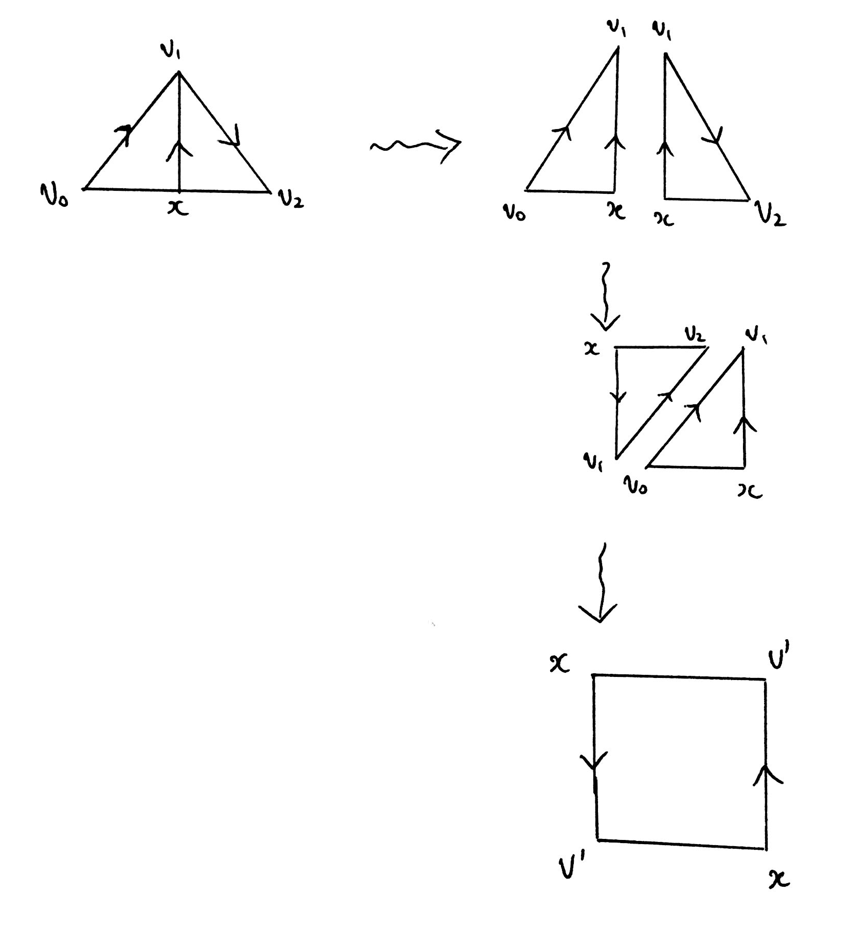
What familiar space is the quotient ![[v_0,v_1,v_2]](https://s0.wp.com/latex.php?latex=%5Bv_0%2Cv_1%2Cv_2%5D&bg=ffffff&fg=1a1a1a&s=0&c=20201002)
This is a question from Hatcher. So if we “glue” two edges of the triangle together, preserving order, we get a Mobius Strip!
Covering map is an open map
We prove a lemma that the covering map 
Let 


There exists 


Topology Puzzle
Assume you are a superman who is very elastic, after making linked rings with your index fingers and thumbs, could you move your hands apart without separating the joined fingertips?

In other words, is it possible to go from (a) to (b) without “breaking” the figure above?
Figure taken from Intuitive Topology (Mathematical World, Vol 4).
The answer is yes!
This is an animation of the solution: https://vk.com/video-9666747_142799479
Topology book for General Audience
Previously I blogged about the book The Shape of Space, here is another book that is also about topology and suitable for a general audience (high school and above)!

Effective Homotopy Method
The main idea of the effective homotopy method is the following: given some Kan simplicial sets 


Representing map of x
Proposition:
(Representing map of 

![f_x:\Delta[n]\to X](https://s0.wp.com/latex.php?latex=f_x%3A%5CDelta%5Bn%5D%5Cto+X&bg=ffffff&fg=1a1a1a&s=0&c=20201002)

Proof:
Let ![(i_0,i_1,\dots,i_k)\in\Delta[n]](https://s0.wp.com/latex.php?latex=%28i_0%2Ci_1%2C%5Cdots%2Ci_k%29%5Cin%5CDelta%5Bn%5D&bg=ffffff&fg=1a1a1a&s=0&c=20201002)


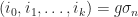


This defines a unique simplicial map 

Minimal Simplicial Sets
Let 


Let 


![\partial\Delta[n]](https://s0.wp.com/latex.php?latex=%5Cpartial%5CDelta%5Bn%5D&bg=ffffff&fg=1a1a1a&s=0&c=20201002)
A fibrant simplicial set is said to be minimal if it has the property that 
Let 


In other words, it means that a fibrant simplicial set is minimal iff for any two elements with all faces but one the same, then the missed face must be the same.
Higher Homotopy Groups
We can generalise the idea to higher homotopy groups as follows.
Let 


The product structure in ![[x]+[x']=[d_1w]](https://s0.wp.com/latex.php?latex=%5Bx%5D%2B%5Bx%27%5D%3D%5Bd_1w%5D&bg=ffffff&fg=1a1a1a&s=0&c=20201002)


Associativity and Path Inverse for Fundamental Groupoids
Continued from Path product and fundamental groupoids
(Associativity). Let 


![(\lambda_1*\lambda_2)*\lambda_3\simeq\lambda_1*(\lambda_2*\lambda_3)\ \text{rel}\ \partial\Delta[1]](https://s0.wp.com/latex.php?latex=%28%5Clambda_1%2A%5Clambda_2%29%2A%5Clambda_3%5Csimeq%5Clambda_1%2A%28%5Clambda_2%2A%5Clambda_3%29%5C+%5Ctext%7Brel%7D%5C+%5Cpartial%5CDelta%5B1%5D&bg=ffffff&fg=1a1a1a&s=0&c=20201002)
Let 


(Path Inverse). Let 

![\lambda*\lambda^{-1}\simeq\epsilon_{\lambda(0)}\ \text{rel}\ \partial\Delta[1]](https://s0.wp.com/latex.php?latex=%5Clambda%2A%5Clambda%5E%7B-1%7D%5Csimeq%5Cepsilon_%7B%5Clambda%280%29%7D%5C+%5Ctext%7Brel%7D%5C+%5Cpartial%5CDelta%5B1%5D&bg=ffffff&fg=1a1a1a&s=0&c=20201002)
Path product and fundamental groupoids
Let ![\sigma_1=(0,1)\in\Delta[1]_1](https://s0.wp.com/latex.php?latex=%5Csigma_1%3D%280%2C1%29%5Cin%5CDelta%5B1%5D_1&bg=ffffff&fg=1a1a1a&s=0&c=20201002)
![\lambda:\Delta[1]\to X](https://s0.wp.com/latex.php?latex=%5Clambda%3A%5CDelta%5B1%5D%5Cto+X&bg=ffffff&fg=1a1a1a&s=0&c=20201002)
![\text{Hom}(\Delta[1],X)\cong X_1](https://s0.wp.com/latex.php?latex=%5Ctext%7BHom%7D%28%5CDelta%5B1%5D%2CX%29%5Ccong+X_1&bg=ffffff&fg=1a1a1a&s=0&c=20201002)


Let 


Homotopy Groups
Let ![\pi_n(X)=[S^n,X]](https://s0.wp.com/latex.php?latex=%5Cpi_n%28X%29%3D%5BS%5En%2CX%5D&bg=ffffff&fg=1a1a1a&s=0&c=20201002)

An element 

Given a spherical element ![S^n=\Delta[n]/\partial\Delta[n]](https://s0.wp.com/latex.php?latex=S%5En%3D%5CDelta%5Bn%5D%2F%5Cpartial%5CDelta%5Bn%5D&bg=ffffff&fg=1a1a1a&s=0&c=20201002)


Path product and fundamental groupoids
Let
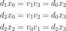
Geometrical Meaning of Matching Faces
Let 


Geometrically, matching faces are faces that “match” along lower-dimensional faces. In other words, they are “adjacent”.

In the 2-simplex, let 


In the 3-simplex, let 


Fibrant Simplicial Set
Let ![f:\Lambda^i[n]\to X](https://s0.wp.com/latex.php?latex=f%3A%5CLambda%5Ei%5Bn%5D%5Cto+X&bg=ffffff&fg=1a1a1a&s=0&c=20201002)
Assume that 
Thus, since 

![g=f_w:\Delta[n]\to X](https://s0.wp.com/latex.php?latex=g%3Df_w%3A%5CDelta%5Bn%5D%5Cto+X&bg=ffffff&fg=1a1a1a&s=0&c=20201002)


Conversely let ![f_{x_j}:\Delta[n-1]\to X](https://s0.wp.com/latex.php?latex=f_%7Bx_j%7D%3A%5CDelta%5Bn-1%5D%5Cto+X&bg=ffffff&fg=1a1a1a&s=0&c=20201002)
![f:\Lambda^i [n]\to X](https://s0.wp.com/latex.php?latex=f%3A%5CLambda%5Ei+%5Bn%5D%5Cto+X&bg=ffffff&fg=1a1a1a&s=0&c=20201002)

commutes for each
By the assumption, there exists an extension ![g:\Delta[n]\to X](https://s0.wp.com/latex.php?latex=g%3A%5CDelta%5Bn%5D%5Cto+X&bg=ffffff&fg=1a1a1a&s=0&c=20201002)
![g|_{\Lambda^i[n]}=f](https://s0.wp.com/latex.php?latex=g%7C_%7B%5CLambda%5Ei%5Bn%5D%7D%3Df&bg=ffffff&fg=1a1a1a&s=0&c=20201002)


