Proof:
We consider 

We consider 

Consider the map from the unit ball 


Hence 
Next, the mapping 

Proof:
We consider
We consider
Consider the map from the unit ball
Hence
Next, the mapping

Proof:
We have that
Since 
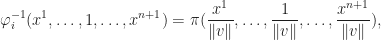
Consider the map
It is clear that 


If 

Note that 

When 


Hence
De Rham Cohomology is a very cool sounding term in advanced math. This blog post is a short introduction on how it is defined.
Also, do check out our presentation on the relation between De Rham Cohomology and physics: De Rham Cohomology.
Definition:
A differential form 


Corollary:
Since 
Definition:
Let 
Let 
Since every exact form is closed, hence 
The de Rham cohomology of
The quotient vector space construction induces an equivalence relation on


The equivalence class of a closed form ![[\omega]](https://s0.wp.com/latex.php?latex=%5B%5Comega%5D&bg=ffffff&fg=1a1a1a&s=0&c=20201002)
Proposition: 
Proof:
Define ![U_1=\{[z^1, z^2]\mid z^1\neq 0\}](https://s0.wp.com/latex.php?latex=U_1%3D%5C%7B%5Bz%5E1%2C+z%5E2%5D%5Cmid+z%5E1%5Cneq+0%5C%7D&bg=ffffff&fg=1a1a1a&s=0&c=20201002)
![U_2=\{[z^1, z^2]\mid z^2\neq 0\}](https://s0.wp.com/latex.php?latex=U_2%3D%5C%7B%5Bz%5E1%2C+z%5E2%5D%5Cmid+z%5E2%5Cneq+0%5C%7D&bg=ffffff&fg=1a1a1a&s=0&c=20201002)

![g_1([z^1, z^2])=\frac{z^2}{z^1}](https://s0.wp.com/latex.php?latex=g_1%28%5Bz%5E1%2C+z%5E2%5D%29%3D%5Cfrac%7Bz%5E2%7D%7Bz%5E1%7D&bg=ffffff&fg=1a1a1a&s=0&c=20201002)
![g_2([z^1, z^2])=\frac{\overline{z^1}}{\overline{z^2}}](https://s0.wp.com/latex.php?latex=g_2%28%5Bz%5E1%2C+z%5E2%5D%29%3D%5Cfrac%7B%5Coverline%7Bz%5E1%7D%7D%7B%5Coverline%7Bz%5E2%7D%7D&bg=ffffff&fg=1a1a1a&s=0&c=20201002)
Let 


Note that 


The transition function
is differentiable of class 
Proposition:

Proof:
Define 


Define 


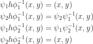
We can check that 


The composite 


We can also compute the transition function explicitly:
Note that 
Define 


We see that 


Similarly, we have a well-defined inverse 


We check that (from our previous workings)
are of class 
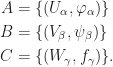
Let 

The tangent space to 

Smooth Manifold
A smooth manifold is a pair 

Topological Manifold
A topological 
1) 


2)
3) 
– an open set 
– an open set 
– a homeomorphism 
Smooth structure
A smooth structure
Smooth Atlas


Source:
Introduction to Smooth Manifolds (Graduate Texts in Mathematics, Vol. 218) by John Lee
Differentiable Manifolds (Modern Birkhäuser Classics) by Lawrence Conlon
These two books are highly recommended books for Differentiable Manifolds. John Lee’s book has almost become the standard book. Its style is similar to Hatcher’s Algebraic Topology, it can be wordy but it has detailed description and explanation of the ideas, so it is good for those learning the material for the first time.
Lawrence Conlon’s book is more concise, and has specialized chapters that link to Algebraic Topology.
Define an equivalence relation on 


Prove
1) 
2) 
3) There is a homeomorphism 
4)
Proof:
1) 

2) Let 


3) Consider 


4) Since 
Equivalence of
Proof:
Reflexive: If 

Symmetry: Let 


Transitivity: Let 

Notation:
Then 


Let 


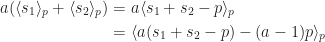
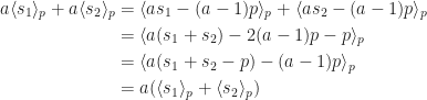
Prove that the operation of linear combination, as in Definition 2.2.7, makes 


Proof:
We verify the axioms of a vector space.
Multiplicative axioms:
*
*
Additive Axioms:
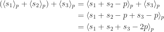
*
*
*
Hence 
*
Distributive Axioms:
*
*
Hence 
If 


Proof:
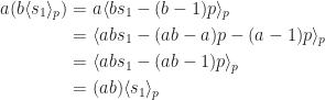
Let 


By choosing 


![\begin{aligned} \phi_2\phi_1^{-1}(x,y)&=\phi_2 g_1^{-1}(x+iy)\\ &=\phi_2([1,x+iy])\\ &=f(\frac{1}{x-iy})\\ &=f(\frac{x+iy}{x^2+y^2})\\ &=(\frac{x}{x^2+y^2},\frac{y}{x^2+y^2}) \end{aligned}](https://s0.wp.com/latex.php?latex=%5Cbegin%7Baligned%7D++%5Cphi_2%5Cphi_1%5E%7B-1%7D%28x%2Cy%29%26%3D%5Cphi_2+g_1%5E%7B-1%7D%28x%2Biy%29%5C%5C++%26%3D%5Cphi_2%28%5B1%2Cx%2Biy%5D%29%5C%5C++%26%3Df%28%5Cfrac%7B1%7D%7Bx-iy%7D%29%5C%5C++%26%3Df%28%5Cfrac%7Bx%2Biy%7D%7Bx%5E2%2By%5E2%7D%29%5C%5C++%26%3D%28%5Cfrac%7Bx%7D%7Bx%5E2%2By%5E2%7D%2C%5Cfrac%7By%7D%7Bx%5E2%2By%5E2%7D%29++%5Cend%7Baligned%7D&bg=ffffff&fg=1a1a1a&s=0&c=20201002)