We let  be a simple
  -algebra. Then
  , the n by n matrix algebra over is simple. In particular if
  is a division algebra, then
  is simple.
Reference: Associative Algebras (Graduate Texts in Mathematics)
We will split our proof into 2 Lemmas.
Lemma 1: If  , then
  .
.
Proof: Let  .
.
 . Therefore
  .
.
 , thus
  . Similarly
  . Thus
  is indeed an ideal of .
Lemma 2 (Tricky part, takes some time to digest): If  , then
  for some .
A technical thing we need to know is the  matrix, which is a n by n matrix with 1 in the (i,j) entry, 0 elsewhere. A key property is that
  if
if  , and 0 otherwise (zero matrix).
The key idea here is that  can be taken to be
  . We can check that is indeed an ideal. We need to know that it is possible to premultiply and postmultiply a given matrix by “elementary matrices” such that any entry of the given matrix is “shifted” to the (1,1) entry. An example will be
  .
.
Let us begin the proof to first show  . Let
. Let  . We write
  . For any
  ,
,

Therefore  . Therefore
  . What we are actually doing here is first pick an arbitrary matrix
  in
in  . Then, we do the “shifting” process to show that any (p,q) entry in can be “shifted” to the (1,1) entry, thus it is inside our ideal . Since any arbitrary (p,q) entry in is inside the ideal , we conclude that is an element of .
Next part is to show  . Let
. Let  . We have
  for all
  . We compute that

Therefore  . We will illustrate what we are doing here by an example in the 2 by 2 case. Let us have
  . Since is in , what we have, by definition of , is that
  ,
,  ,
,  ,
,  are all in . We then proceed to “shift” them all into their correct positions: ,
  ,
,  ,
,  , all of which are still in the ideal . is the sum of all of them, thus also in .
Final Conclusion
Since is simple, its ideals are 0 and itself. Thus, the ideals of will be also the 0 matrix and itself, and thus is simple. A division algebra is simple (Any ideal containing a nonzero element  , when multiplied by its inverse will give 1. Thus the ideal will contain 1 and thus the entire ring ), thus is also simple.


 by Peter Lax. This book is ideal for a second course in Functional Analysis. For a first course in Functional Analysis, I would recommend Kreyszig, which is listed on my
  is convex, so is
  .
. be a collection of convex subsets that is totally ordered by inclusion. Then their union
  is convex.
 belong to
  ,
,  also belong to
  .
. and
and  be the two convex subsets. Let
  and
and  be points in
![\begin{aligned} a(x_1+y_1)+(1-a)(x_2+y_2)&=ax_1+ay_1+x_2+y_2-ax_2-ay_2\\ &=[ax_1+(1-a)x_2]+[ay_1+(1-a)y_2]\\ &\in C_1+C_2 \end{aligned}](https://s0.wp.com/latex.php?latex=%5Cbegin%7Baligned%7D++++a%28x_1%2By_1%29%2B%281-a%29%28x_2%2By_2%29%26%3Dax_1%2Bay_1%2Bx_2%2By_2-ax_2-ay_2%5C%5C++++%26%3D%5Bax_1%2B%281-a%29x_2%5D%2B%5Bay_1%2B%281-a%29y_2%5D%5C%5C++++%26%5Cin+C_1%2BC_2++++%5Cend%7Baligned%7D&bg=ffffff&fg=1a1a1a&s=0&c=20201002)
 and this algebraic observation:
  .
. .
.  for all
  , thus
  .
. , where
  . Let
. Let  ,
,  , then either
  or
or  . If
. If  . Similarly for the other case
  .
. exists. We can only talk about the pre-image.
 .
.  and
and  .
. .
. .
. .
. , under the transformation
  , where
  are of the same sign.
 , note that by arguments similar to
  .
. , upon completing the square, becomes
 — Circle 1
 is transformed into:
 — Circle 2
 and
and  to the vertical strip
  .
. . Now we are in the situation of our above analysis, thus inversion
  . The map
  (reflection), followed by
  , finally finishing up with a scaling of factor 2 brings us to the vertical strip desired.
 to the very nice strip
  .
. in a subsequent blog post.

 and
and  be
be  . The source of the material will primarily come from
  (by Dummit and Foote) which is a highly recommended Algebra book for undergraduates.
 of elements
  and
and  .
. -module over
  (also called module of the formal linear combinations of elements of


 under the transformation
  )
) ,
,  .
. ,
,  . From the equation
  , we can conclude that
  .
. , which is the equation of a circle centered at
  with radius
  . When
  , the equation of the circle is
  . As
. As  . It is a very unique book, in the sense that it is aimed at high school students, but even a undergraduate or graduate student can benefit from it. It has a lot of diagrams, that are missing in most textbooks, presumably because it takes a lot of effort to draw a mathematical (3D) diagram.

 that induces isomorphisms
  for all
  and all choices of basepoint
  .
. such that
  and
and  . The spaces
  are called homotopy equivalent.
 and a weak homotopy equivalence
  . This map
  with nonempty connected intersection
  . If
. If  is m-connected and
  is n-connected,
  , then the map
  induced by inclusion is an isomorphism for
  and a surjection for
  .
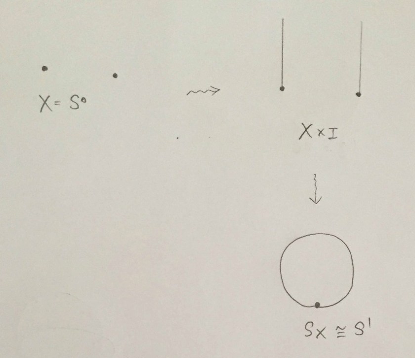
. is the quotient of
  obtained by collapsing
  to one point and
  to another point.
 is the union of all line segments joining points of
  , when
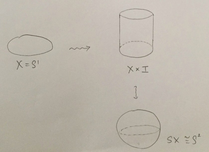
  with the two “suspension points” at the north and south poles of
  , the points
  .
.
 , with
  , and
, and  are complex constants, is called a linear fractional transformation, or Mobius transformation.
 ,
,  ,
,  onto the points
  ,
,  ,
,  . (Question taken from
 ,
,  and
and  .
. :
:  ,
,  ,
,  . Substituting back into the Mobius Transformation gives us the answer.
 (where
  and
and  are open sets) is an analytic function such that there exists another analytic function
  , satisfying
  and
and  .
.

 of CW pairs can be deformed through maps
  to a cellular map
  .
. is a map from
  under
under  means that
  to be cellular. We then use the
  have dimension greater than
  . In particular the pair
  is n-connected, hence the inclusion
  induces isomorphisms on
  for
for  and a surjection on
  .
. for
for  .
. with
with  , thus the map is homotopic to a cellular map of pairs
  . Since all the cells in
  . This proves that the CW pair
 (since
  ). Thus
  is surjective. Since

 ,
,  be holomorphic inside and on a simple closed contour
  on
on  have the same number of zeroes (counting multiplicities) inside
  in the annulus
  .
. be the unit circle
 has 2 zeroes in
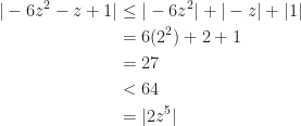
  be the circle
 . Chose
  sufficiently large so that on the circle
  ,
,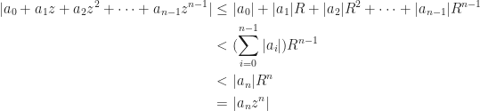
 has
has 

 , where
  , where
  is an odd prime.
 ,
,  and
and  .
. in
in  is
is ![Q(\sqrt[p]{2},\omega)](https://s0.wp.com/latex.php?latex=Q%28%5Csqrt%5Bp%5D%7B2%7D%2C%5Comega%29&bg=ffffff&fg=1a1a1a&s=0&c=20201002) , where
, where  is a primitive p-th root of unity. The roots of
 ![\sqrt[p]2, \sqrt[p]2\omega, \sqrt[p]2\omega^2, \dots, \sqrt[p]2\omega^{p-1}](https://s0.wp.com/latex.php?latex=%5Csqrt%5Bp%5D2%2C+%5Csqrt%5Bp%5D2%5Comega%2C+%5Csqrt%5Bp%5D2%5Comega%5E2%2C+%5Cdots%2C+%5Csqrt%5Bp%5D2%5Comega%5E%7Bp-1%7D&bg=ffffff&fg=1a1a1a&s=0&c=20201002) .
.![\sqrt[p]2](https://s0.wp.com/latex.php?latex=%5Csqrt%5Bp%5D2&bg=ffffff&fg=1a1a1a&s=0&c=20201002) and
and ![\omega=\frac{\sqrt[p]2\omega^2}{\sqrt[p]2\omega}](https://s0.wp.com/latex.php?latex=%5Comega%3D%5Cfrac%7B%5Csqrt%5Bp%5D2%5Comega%5E2%7D%7B%5Csqrt%5Bp%5D2%5Comega%7D&bg=ffffff&fg=1a1a1a&s=0&c=20201002) . Thus
. Thus ![\mathbb{Q}(\sqrt[p]2,\omega)\subseteq K](https://s0.wp.com/latex.php?latex=%5Cmathbb%7BQ%7D%28%5Csqrt%5Bp%5D2%2C%5Comega%29%5Csubseteq+K&bg=ffffff&fg=1a1a1a&s=0&c=20201002) .
.![\mathbb{Q}(\sqrt[p]2,\omega)](https://s0.wp.com/latex.php?latex=%5Cmathbb%7BQ%7D%28%5Csqrt%5Bp%5D2%2C%5Comega%29&bg=ffffff&fg=1a1a1a&s=0&c=20201002) contains all the roots of
contains all the roots of ![\mathbb{Q}(\sqrt[p]2, \omega)](https://s0.wp.com/latex.php?latex=%5Cmathbb%7BQ%7D%28%5Csqrt%5Bp%5D2%2C+%5Comega%29&bg=ffffff&fg=1a1a1a&s=0&c=20201002) . Thus
. Thus ![K\subseteq\mathbb{Q}(\sqrt[p]2,\omega)](https://s0.wp.com/latex.php?latex=K%5Csubseteq%5Cmathbb%7BQ%7D%28%5Csqrt%5Bp%5D2%2C%5Comega%29&bg=ffffff&fg=1a1a1a&s=0&c=20201002) , since
, since ![K=\mathbb{Q}(\sqrt[p]2, \omega)](https://s0.wp.com/latex.php?latex=K%3D%5Cmathbb%7BQ%7D%28%5Csqrt%5Bp%5D2%2C+%5Comega%29&bg=ffffff&fg=1a1a1a&s=0&c=20201002) .
.![|Gal(K/\mathbb{Q})|=[K:\mathbb{Q}]](https://s0.wp.com/latex.php?latex=%7CGal%28K%2F%5Cmathbb%7BQ%7D%29%7C%3D%5BK%3A%5Cmathbb%7BQ%7D%5D&bg=ffffff&fg=1a1a1a&s=0&c=20201002) . Since
. Since ![[\mathbb{Q}(\sqrt[p]2):\mathbb{Q}]=p](https://s0.wp.com/latex.php?latex=%5B%5Cmathbb%7BQ%7D%28%5Csqrt%5Bp%5D2%29%3A%5Cmathbb%7BQ%7D%5D%3Dp&bg=ffffff&fg=1a1a1a&s=0&c=20201002) (minimal polynomial
(minimal polynomial  ), and
 ![[\mathbb{Q}(\omega):\mathbb{Q}]=p-1](https://s0.wp.com/latex.php?latex=%5B%5Cmathbb%7BQ%7D%28%5Comega%29%3A%5Cmathbb%7BQ%7D%5D%3Dp-1&bg=ffffff&fg=1a1a1a&s=0&c=20201002) (minimal polynomial the cyclotomic polynomial
(minimal polynomial the cyclotomic polynomial  ), thus
  . Here we have used the lemma that suppose
 ![[F(\alpha):F]=m](https://s0.wp.com/latex.php?latex=%5BF%28%5Calpha%29%3AF%5D%3Dm&bg=ffffff&fg=1a1a1a&s=0&c=20201002) and
and ![[F(\beta):F]=n](https://s0.wp.com/latex.php?latex=%5BF%28%5Cbeta%29%3AF%5D%3Dn&bg=ffffff&fg=1a1a1a&s=0&c=20201002) with
with  , then
 ![[F(\alpha,\beta):F]=mn](https://s0.wp.com/latex.php?latex=%5BF%28%5Calpha%2C%5Cbeta%29%3AF%5D%3Dmn&bg=ffffff&fg=1a1a1a&s=0&c=20201002) .
. be an element of the Galois group.
 ![\sigma(\sqrt[p]2)](https://s0.wp.com/latex.php?latex=%5Csigma%28%5Csqrt%5Bp%5D2%29&bg=ffffff&fg=1a1a1a&s=0&c=20201002) can possibly be
can possibly be ![\sqrt[p]2, \sqrt[p]\omega, \dots, \sqrt[p]2\omega^{p-1}](https://s0.wp.com/latex.php?latex=%5Csqrt%5Bp%5D2%2C+%5Csqrt%5Bp%5D%5Comega%2C+%5Cdots%2C+%5Csqrt%5Bp%5D2%5Comega%5E%7Bp-1%7D&bg=ffffff&fg=1a1a1a&s=0&c=20201002) , a total of
, a total of  , a total of
  choices. All these total up to
  elements, which is exactly the size of the Galois group.
 is described by how its elements act on the generators. For a more concrete representation, we can actually prove that the Galois group above is isomorphic to the group of matrices
  , where
  ,
,  . We denote the group of matrices as
  , mapping
  to
to ![\sigma_{a,b}(\sqrt[p]2)=\sqrt[p]2\omega^b](https://s0.wp.com/latex.php?latex=%5Csigma_%7Ba%2Cb%7D%28%5Csqrt%5Bp%5D2%29%3D%5Csqrt%5Bp%5D2%5Comega%5Eb&bg=ffffff&fg=1a1a1a&s=0&c=20201002) ,
,  .
. is bijective. To see it is a homomorphism, we compute
  .
. for all
  , we have an even stronger conclusion:
  , the homotopy may be taken to be stationary on
  , then
  .
. and
and  with their canonical CW-structure, with one 0-cell each, and with one n-cell for
 ![[f]\in\pi_n(S^k)](https://s0.wp.com/latex.php?latex=%5Bf%5D%5Cin%5Cpi_n%28S%5Ek%29&bg=ffffff&fg=1a1a1a&s=0&c=20201002) , where
, where  is a base-point preserving map. By the Cellular Approximation Theorem,
  be a uniformly bounded and equicontinuous sequence of real-valued continuous functions defined on a closed and bounded interval
 ![[a,b]](https://s0.wp.com/latex.php?latex=%5Ba%2Cb%5D&bg=ffffff&fg=1a1a1a&s=0&c=20201002) . Then there exists a subsequence
. Then there exists a subsequence  that converges uniformly.
 for all
  and all
 ![x\in [a,b]](https://s0.wp.com/latex.php?latex=x%5Cin+%5Ba%2Cb%5D&bg=ffffff&fg=1a1a1a&s=0&c=20201002) . The sequence is equicontinous if, for all
. The sequence is equicontinous if, for all  , there exists
  such that
  whenever
  for all functions
  (depending solely on
  ) works for the entire family of functions.
![g:[0,1]\times [0,1]\to [0,1]](https://s0.wp.com/latex.php?latex=g%3A%5B0%2C1%5D%5Ctimes+%5B0%2C1%5D%5Cto+%5B0%2C1%5D&bg=ffffff&fg=1a1a1a&s=0&c=20201002) be a continuous function and let
be a continuous function and let  be a sequence of functions such that
![f:[0,1]\to\mathbb{R}](https://s0.wp.com/latex.php?latex=f%3A%5B0%2C1%5D%5Cto%5Cmathbb%7BR%7D&bg=ffffff&fg=1a1a1a&s=0&c=20201002) such that
such that  for all
 ![x\in [0,1]](https://s0.wp.com/latex.php?latex=x%5Cin+%5B0%2C1%5D&bg=ffffff&fg=1a1a1a&s=0&c=20201002) .
.
 ,
,
 ,
,  .
. and
and  ,
,
 , then whenever
  . Thus the sequence is indeed equicontinuous.
 .
.


![\mathbb{Z}[i]](https://s0.wp.com/latex.php?latex=%5Cmathbb%7BZ%7D%5Bi%5D&bg=ffffff&fg=1a1a1a&s=0&c=20201002) are the set of complex numbers of the form
are the set of complex numbers of the form  , with
  integers. Originally discovered and studied by Gauss, the Gaussian Integers are useful in number theory, for instance they can be used to prove that
 ![\mathbb{Z}[i]/I](https://s0.wp.com/latex.php?latex=%5Cmathbb%7BZ%7D%5Bi%5D%2FI&bg=ffffff&fg=1a1a1a&s=0&c=20201002) is finite.
is finite. for some nonzero
 ![\alpha\in\mathbb{Z}[i]](https://s0.wp.com/latex.php?latex=%5Calpha%5Cin%5Cmathbb%7BZ%7D%5Bi%5D&bg=ffffff&fg=1a1a1a&s=0&c=20201002) . Let
. Let ![\beta\in\mathbb{Z}[i]](https://s0.wp.com/latex.php?latex=%5Cbeta%5Cin%5Cmathbb%7BZ%7D%5Bi%5D&bg=ffffff&fg=1a1a1a&s=0&c=20201002) .
. with
with  or
or  . We also note that
  .
.![\begin{aligned}\mathbb{Z}[i]/I&=\{\beta+I\mid\beta\in\mathbb{Z}[i]\}\\ &=\{r+I\mid r\in\mathbb{Z}[i],N(r)<N(\alpha)\} \end{aligned}](https://s0.wp.com/latex.php?latex=%5Cbegin%7Baligned%7D%5Cmathbb%7BZ%7D%5Bi%5D%2FI%26%3D%5C%7B%5Cbeta%2BI%5Cmid%5Cbeta%5Cin%5Cmathbb%7BZ%7D%5Bi%5D%5C%7D%5C%5C++++%26%3D%5C%7Br%2BI%5Cmid+r%5Cin%5Cmathbb%7BZ%7D%5Bi%5D%2CN%28r%29%3CN%28%5Calpha%29%5C%7D++++%5Cend%7Baligned%7D&bg=ffffff&fg=1a1a1a&s=0&c=20201002) .
.![r\in\mathbb{Z}[i]](https://s0.wp.com/latex.php?latex=r%5Cin%5Cmathbb%7BZ%7D%5Bi%5D&bg=ffffff&fg=1a1a1a&s=0&c=20201002) with
with  of an arbitrary collection of path-connected spaces
  there are isomorphisms
  for all
  is the same thing as a collection of maps
  . Taking
  gives the result.
 , which is the result for a product of two spaces. The general result then follows by induction.
 ,
, ![\psi([f])=([f_1],[f_2])](https://s0.wp.com/latex.php?latex=%5Cpsi%28%5Bf%5D%29%3D%28%5Bf_1%5D%2C%5Bf_2%5D%29&bg=ffffff&fg=1a1a1a&s=0&c=20201002) .
. ,
,  ,
,  where
where  are the projection maps.
![\psi ([f]+[g])=\psi([f])+\psi([g])](https://s0.wp.com/latex.php?latex=%5Cpsi+%28%5Bf%5D%2B%5Bg%5D%29%3D%5Cpsi%28%5Bf%5D%29%2B%5Cpsi%28%5Bg%5D%29&bg=ffffff&fg=1a1a1a&s=0&c=20201002) , thus
, thus  is a homomorphism.
 ,
, ![\phi([g_1],[g_2])=[g]](https://s0.wp.com/latex.php?latex=%5Cphi%28%5Bg_1%5D%2C%5Bg_2%5D%29%3D%5Bg%5D&bg=ffffff&fg=1a1a1a&s=0&c=20201002) where
where  ,
,  .
. . Show that the set
  is measurable.
 . This is popularly known as the graph of a function. Without loss of generality, we may assume that
  , where we split the function into two nonnegative parts.
 ,
,  .
. , where
  indicates outer measure.
 , where
  are disjoint.
 , we can conclude
  and thus
  is measurable (and has measure zero).
 , we partition
  into countable union of sets
  each with finite measure. By the same analysis, each
  is measurable (and has measure zero). Thus
  is a countable union of measurable sets and thus is measurable (has measure zero).
 is normal in a group
  is to show that “left coset = right coset”, i.e.
  for all
  . Variations of this method include showing that
  ,
,  , and so on.
![[G:H]=p](https://s0.wp.com/latex.php?latex=%5BG%3AH%5D%3Dp&bg=ffffff&fg=1a1a1a&s=0&c=20201002) , where
, where  . Show that
  by left translation.
 ,
,  .
. , and
, and  .
. . Let
. Let  .
.  for all
  , i.e.
  for all
  . In particular when
  ,
,  . This means that
  . So we have
  .
. , i.e.
 ![[H:\ker\sigma]>1](https://s0.wp.com/latex.php?latex=%5BH%3A%5Cker%5Csigma%5D%3E1&bg=ffffff&fg=1a1a1a&s=0&c=20201002) . Let
. Let  be a prime divisor of
 ![[H:\ker\sigma]](https://s0.wp.com/latex.php?latex=%5BH%3A%5Cker%5Csigma%5D&bg=ffffff&fg=1a1a1a&s=0&c=20201002) .
.![[G:\ker\sigma]=[G:H][H:\ker\sigma]=p[H:\ker\sigma]](https://s0.wp.com/latex.php?latex=%5BG%3A%5Cker%5Csigma%5D%3D%5BG%3AH%5D%5BH%3A%5Cker%5Csigma%5D%3Dp%5BH%3A%5Cker%5Csigma%5D&bg=ffffff&fg=1a1a1a&s=0&c=20201002)
 . By Lagrange’s Theorem,
 ![[G:\ker\sigma]\mid p!](https://s0.wp.com/latex.php?latex=%5BG%3A%5Cker%5Csigma%5D%5Cmid+p%21&bg=ffffff&fg=1a1a1a&s=0&c=20201002) , i.e.
, i.e. ![p[H:\ker\sigma]\mid p!](https://s0.wp.com/latex.php?latex=p%5BH%3A%5Cker%5Csigma%5D%5Cmid+p%21&bg=ffffff&fg=1a1a1a&s=0&c=20201002) . This implies
. This implies ![[H:\ker\sigma]\mid(p-1)!](https://s0.wp.com/latex.php?latex=%5BH%3A%5Cker%5Csigma%5D%5Cmid%28p-1%29%21&bg=ffffff&fg=1a1a1a&s=0&c=20201002) . Finally,
. Finally,  implies
  .
.![q\mid [H:\ker\sigma]](https://s0.wp.com/latex.php?latex=q%5Cmid+%5BH%3A%5Cker%5Csigma%5D&bg=ffffff&fg=1a1a1a&s=0&c=20201002) implies
implies ![q\mid[G:\ker\sigma]=\frac{|G|}{|\ker\sigma|}](https://s0.wp.com/latex.php?latex=q%5Cmid%5BG%3A%5Cker%5Csigma%5D%3D%5Cfrac%7B%7CG%7C%7D%7B%7C%5Cker%5Csigma%7C%7D&bg=ffffff&fg=1a1a1a&s=0&c=20201002) which implies
which implies  .
. and therefore
  we can conclude that the polynomial
  has no roots on the circle
  when
when  .
. induces isomorphisms
  for all
  .
. is a homomorphism and also bijective (surjective and injective).
![p_*([f]):=[pf]](https://s0.wp.com/latex.php?latex=p_%2A%28%5Bf%5D%29%3A%3D%5Bpf%5D&bg=ffffff&fg=1a1a1a&s=0&c=20201002)
![p_*([f]+[g])=[p(f+g)]](https://s0.wp.com/latex.php?latex=p_%2A%28%5Bf%5D%2B%5Bg%5D%29%3D%5Bp%28f%2Bg%29%5D&bg=ffffff&fg=1a1a1a&s=0&c=20201002)
![p(f+g)(s_1,s_2,\dots,s_n)=\begin{cases}pf(2s_1,s_2,\dots,s_n)&s_1\in[0,\frac 12]\\ pg(2s_1-1,s_2,\dots,s_n)&s_1\in[\frac 12,1] \end{cases}](https://s0.wp.com/latex.php?latex=p%28f%2Bg%29%28s_1%2Cs_2%2C%5Cdots%2Cs_n%29%3D%5Cbegin%7Bcases%7Dpf%282s_1%2Cs_2%2C%5Cdots%2Cs_n%29%26s_1%5Cin%5B0%2C%5Cfrac+12%5D%5C%5C++++pg%282s_1-1%2Cs_2%2C%5Cdots%2Cs_n%29%26s_1%5Cin%5B%5Cfrac+12%2C1%5D++++%5Cend%7Bcases%7D&bg=ffffff&fg=1a1a1a&s=0&c=20201002)
![p_*[f]+p_*[g]=[pf]+[pg]](https://s0.wp.com/latex.php?latex=p_%2A%5Bf%5D%2Bp_%2A%5Bg%5D%3D%5Bpf%5D%2B%5Bpg%5D&bg=ffffff&fg=1a1a1a&s=0&c=20201002)
![(pf+pg)(s_1,s_2,\dots,s_n)= \begin{cases}pf(2s_1,s_2,\dots,s_n)&s_1\in[0,\frac 12]\\ pg(2s_1-1,s_2,\dots,s_n)&s_1\in[\frac 12,1] \end{cases}](https://s0.wp.com/latex.php?latex=%28pf%2Bpg%29%28s_1%2Cs_2%2C%5Cdots%2Cs_n%29%3D++++%5Cbegin%7Bcases%7Dpf%282s_1%2Cs_2%2C%5Cdots%2Cs_n%29%26s_1%5Cin%5B0%2C%5Cfrac+12%5D%5C%5C++++pg%282s_1-1%2Cs_2%2C%5Cdots%2Cs_n%29%26s_1%5Cin%5B%5Cfrac+12%2C1%5D++++%5Cend%7Bcases%7D&bg=ffffff&fg=1a1a1a&s=0&c=20201002) , which we can see is the same.
, which we can see is the same. with
with  of
of  .
.![[f]\in\pi_n(X,x_0)](https://s0.wp.com/latex.php?latex=%5Bf%5D%5Cin%5Cpi_n%28X%2Cx_0%29&bg=ffffff&fg=1a1a1a&s=0&c=20201002) , where
, where  . Since
  . Thus
  . By Proposition 1.33, a lift
  of
of  .
.![\boxed{p_*[\tilde{f}]=[p\tilde{f}]=[f]}](https://s0.wp.com/latex.php?latex=%5Cboxed%7Bp_%2A%5B%5Ctilde%7Bf%7D%5D%3D%5Bp%5Ctilde%7Bf%7D%5D%3D%5Bf%5D%7D&bg=ffffff&fg=1a1a1a&s=0&c=20201002) . Hence
. Hence ![[\tilde{f}_0]\in\ker p_*](https://s0.wp.com/latex.php?latex=%5B%5Ctilde%7Bf%7D_0%5D%5Cin%5Cker+p_%2A&bg=ffffff&fg=1a1a1a&s=0&c=20201002) , where
, where  with a homotopy
  of
of  to the trivial loop
  .
. of
of  that lifts
  , i.e.
  . There is a lifted homotopy of loops
  starting with
 ![[\tilde{f}_0]=0](https://s0.wp.com/latex.php?latex=%5B%5Ctilde%7Bf%7D_0%5D%3D0&bg=ffffff&fg=1a1a1a&s=0&c=20201002) in
in  and thus
  -complex of the Klein Bottle.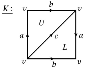
 .
. , the free group generated by the vertex
  , because there is only one vertex!
 . Thus
  .
. .
. .
.  ,
,  . To learn more about calculating
  , check out the diagram on page 105 of Hatcher.
 , where we got
  from adding the two previous generators
  .
. .
. , implies that
  , thus
  , thus is not a generator of
  .
.  implies that
  , which gives us the
  part.
part. , and also for
  ,
,  since there are no simplices of dimension greater than or equal to 3. Thus, the second homology group onwards are all zero.
 , then for any
  , there exists
  such that
  .
.![g:[0,1]\to\mathbb{R}](https://s0.wp.com/latex.php?latex=g%3A%5B0%2C1%5D%5Cto%5Cmathbb%7BR%7D&bg=ffffff&fg=1a1a1a&s=0&c=20201002) ,
,  . By the Mean Value Theorem for one variable, there exists
  such that
  , i.e.
 . Here we are using the chain rule for multivariable calculus to get:
  .
. , then
  as required.

 are increasing functions on [0,1]. Thus by Jordan’s Theorem,
  is a function of bounded variation, but it is certainly not continuous on [0,1]!

 ), real projective plane (
 ), and the Klein bottle (
 , for
, for 
 (Here n-Torus refers to the n-dimensional torus, not the Torus with n holes)
 (usual torus with one hole in 2 dimensions)

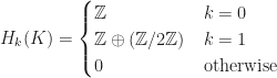
 . Higher homology groups are zero.


 that is a covering map. Since there are many covering spaces, we will list the universal cover instead.
 is the universal cover of the unit circle
 is the universal cover of
  is universal cover of real projective plane
  .
. . There exists an open interval
  containing
  be the maximal open interval in
  . (The existence of
  and
and  then
then  is an open interval in
  . Upon discarding the “repeated” intervals in the union above, we get that
 is an integral domain.
 .
. is a prime ideal of
  is an integral domain. (
 by the Third Isomorphism Theorem. )

