An analytic isomorphism 


An analytic isomorphism
Source: http://www.theliberatedmathematician.com/2015/12/why-i-do-not-talk-about-math/
A honest opinion on the nature of mathematical conversations, by this blog post author Piper Harron. (Also see our previous blog post on her interesting PhD Thesis) Very interesting read, for those who are in the mathematical community.
For those interested in Secondary Level (O Level) Chinese Tuition, do check out http://chinesetuition88.com/.
The tutor (Ms Gao) will be taking in a few more students in 2016 for Chinese Tuition. Do check out http://chinesetuition88.com/ for more info!
(This is Example 4.11 in Hatcher’s book).
Cellular Approximation for Pairs: Every map 


What “map of CW pairs” mean, is that 


First, we use the ordinary Cellular Approximation Theorem to deform the restriction 
We use this to prove a corollary: A CW pair 


First we note that being n-connected means that the space is non-empty, path-connected, and the first n homotopy groups are trivial, i.e. 

Proof: First, we apply cellular approximation to maps 


Consider the long exact sequence of the pair
Since it is an exact sequence, the image of any map equals the kernel of the next. Thus, 


This is the most “unique” PhD thesis I have ever seen. Very special, and humorous to read, and coming from the most elite institution Princeton, under the guidance of Fields Medalist Manjul Bhargava.
Piper Harron is a mathematician who is very happy to be here, and yes, is having a great time, despite the fact that she is standing alone awkwardly by the food table hoping nobody will talk to her.
Piper, would you care to write a mathbabe post describing your thesis, and yourself, and anything else you’d care to mention?
When Cathy (Cathy? mathbabe?) asked if I would like to write a mathbabe post describing my thesis, and myself, and anything else I’d care to mention, I said “sure!” because that is objectively the right answer. I then immediately plunged into despair.
Describe my thesis? My thesis is this thing that was initially going to be a grenade launched at my ex-prison, for better or for worse, and instead turned into some kind of positive seed bomb where flowers have sprouted beside the foundations I thought I wanted to crumble…
View original post 649 more words
The WordPress.com stats helper monkeys prepared a 2015 annual report for this blog.

Here’s an excerpt:
The Louvre Museum has 8.5 million visitors per year. This blog was viewed about 170,000 times in 2015. If it were an exhibit at the Louvre Museum, it would take about 7 days for that many people to see it.
This blog post is on Rouche’s Theorem and some applications, namely counting the number of zeroes in an annulus, and the fundamental theorem of algebra.
Rouche’s Theorem: Let 


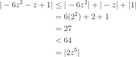
Rouche’s Theorem is useful for scenarios like this: Determine the number of zeroes, counting multiplicities, of the polynomial 

Solution:
Let 

on
Since 
Let 
on
Therefore
We do a computer check using Wolfram Alpha (http://www.wolframalpha.com/input/?i=2z%5E5-6z%5E2-z%2B1%3D0). The moduli of the five roots are (to 3 significant figures): 0.489, 0.335, 1.46, 1.45, 1.45. This confirms that 3 of the zeroes are in the given annulus.
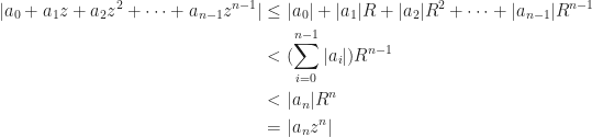
Rouche’s Theorem provides a rather short proof of the Fundamental Theorem of Algebra: Every degree n polynomial with complex coefficients has exactly n roots, counting multiplicities.
Proof: Let 


Since 

Just watched Star Wars: The Force Awakens, here is my review on it. Overall a good movie, enjoyed watching it. The storyline and lightsaber duels are a bit weak in my opinion. How Rey, an untrained person holding a lightsaber for the first time, managed to defeat Kylo Ren with his crossguard lightsaber remains a mystery to me. My favorite episode remains Episode 1: The Phantom Menace.
Many mysteries remain unanswered, like the identities of Rey and Snoke. Looking forward to the next episode.
Something I find very interesting is the Ball Droid BB-8. Something even more interesting about the droid is that it is not CGI effects, it is a real prop. How the head of BB-8 is being attached to the body seems to be via strong magnets.
The toy-version of BB-8 is being sold on Amazon, a possible gift idea for those who are Star Wars fans. Sphero BB-8 App-Enabled Droid
This post is about the Galois group of 


First we show that the polynomial 


Next, we show that the splitting field 

![Q(\sqrt[p]{2},\omega)](https://s0.wp.com/latex.php?latex=Q%28%5Csqrt%5Bp%5D%7B2%7D%2C%5Comega%29&bg=ffffff&fg=1a1a1a&s=0&c=20201002)

![\sqrt[p]2, \sqrt[p]2\omega, \sqrt[p]2\omega^2, \dots, \sqrt[p]2\omega^{p-1}](https://s0.wp.com/latex.php?latex=%5Csqrt%5Bp%5D2%2C+%5Csqrt%5Bp%5D2%5Comega%2C+%5Csqrt%5Bp%5D2%5Comega%5E2%2C+%5Cdots%2C+%5Csqrt%5Bp%5D2%5Comega%5E%7Bp-1%7D&bg=ffffff&fg=1a1a1a&s=0&c=20201002)
The splitting field ![\sqrt[p]2](https://s0.wp.com/latex.php?latex=%5Csqrt%5Bp%5D2&bg=ffffff&fg=1a1a1a&s=0&c=20201002)
![\omega=\frac{\sqrt[p]2\omega^2}{\sqrt[p]2\omega}](https://s0.wp.com/latex.php?latex=%5Comega%3D%5Cfrac%7B%5Csqrt%5Bp%5D2%5Comega%5E2%7D%7B%5Csqrt%5Bp%5D2%5Comega%7D&bg=ffffff&fg=1a1a1a&s=0&c=20201002)
![\mathbb{Q}(\sqrt[p]2,\omega)\subseteq K](https://s0.wp.com/latex.php?latex=%5Cmathbb%7BQ%7D%28%5Csqrt%5Bp%5D2%2C%5Comega%29%5Csubseteq+K&bg=ffffff&fg=1a1a1a&s=0&c=20201002)
On the other hand, ![\mathbb{Q}(\sqrt[p]2,\omega)](https://s0.wp.com/latex.php?latex=%5Cmathbb%7BQ%7D%28%5Csqrt%5Bp%5D2%2C%5Comega%29&bg=ffffff&fg=1a1a1a&s=0&c=20201002)
![\mathbb{Q}(\sqrt[p]2, \omega)](https://s0.wp.com/latex.php?latex=%5Cmathbb%7BQ%7D%28%5Csqrt%5Bp%5D2%2C+%5Comega%29&bg=ffffff&fg=1a1a1a&s=0&c=20201002)
![K\subseteq\mathbb{Q}(\sqrt[p]2,\omega)](https://s0.wp.com/latex.php?latex=K%5Csubseteq%5Cmathbb%7BQ%7D%28%5Csqrt%5Bp%5D2%2C%5Comega%29&bg=ffffff&fg=1a1a1a&s=0&c=20201002)
![K=\mathbb{Q}(\sqrt[p]2, \omega)](https://s0.wp.com/latex.php?latex=K%3D%5Cmathbb%7BQ%7D%28%5Csqrt%5Bp%5D2%2C+%5Comega%29&bg=ffffff&fg=1a1a1a&s=0&c=20201002)
The next part involves determining the Galois group of ![|Gal(K/\mathbb{Q})|=[K:\mathbb{Q}]](https://s0.wp.com/latex.php?latex=%7CGal%28K%2F%5Cmathbb%7BQ%7D%29%7C%3D%5BK%3A%5Cmathbb%7BQ%7D%5D&bg=ffffff&fg=1a1a1a&s=0&c=20201002)
![[\mathbb{Q}(\sqrt[p]2):\mathbb{Q}]=p](https://s0.wp.com/latex.php?latex=%5B%5Cmathbb%7BQ%7D%28%5Csqrt%5Bp%5D2%29%3A%5Cmathbb%7BQ%7D%5D%3Dp&bg=ffffff&fg=1a1a1a&s=0&c=20201002)

![[\mathbb{Q}(\omega):\mathbb{Q}]=p-1](https://s0.wp.com/latex.php?latex=%5B%5Cmathbb%7BQ%7D%28%5Comega%29%3A%5Cmathbb%7BQ%7D%5D%3Dp-1&bg=ffffff&fg=1a1a1a&s=0&c=20201002)


![[F(\alpha):F]=m](https://s0.wp.com/latex.php?latex=%5BF%28%5Calpha%29%3AF%5D%3Dm&bg=ffffff&fg=1a1a1a&s=0&c=20201002)
![[F(\beta):F]=n](https://s0.wp.com/latex.php?latex=%5BF%28%5Cbeta%29%3AF%5D%3Dn&bg=ffffff&fg=1a1a1a&s=0&c=20201002)

![[F(\alpha,\beta):F]=mn](https://s0.wp.com/latex.php?latex=%5BF%28%5Calpha%2C%5Cbeta%29%3AF%5D%3Dmn&bg=ffffff&fg=1a1a1a&s=0&c=20201002)
What the Galois group does is it permutes the roots of 
![\sigma(\sqrt[p]2)](https://s0.wp.com/latex.php?latex=%5Csigma%28%5Csqrt%5Bp%5D2%29&bg=ffffff&fg=1a1a1a&s=0&c=20201002)
![\sqrt[p]2, \sqrt[p]\omega, \dots, \sqrt[p]2\omega^{p-1}](https://s0.wp.com/latex.php?latex=%5Csqrt%5Bp%5D2%2C+%5Csqrt%5Bp%5D%5Comega%2C+%5Cdots%2C+%5Csqrt%5Bp%5D2%5Comega%5E%7Bp-1%7D&bg=ffffff&fg=1a1a1a&s=0&c=20201002)


The above Galois group 


To show the isomorphism, we define a map 

Notation: ![\sigma_{a,b}(\sqrt[p]2)=\sqrt[p]2\omega^b](https://s0.wp.com/latex.php?latex=%5Csigma_%7Ba%2Cb%7D%28%5Csqrt%5Bp%5D2%29%3D%5Csqrt%5Bp%5D2%5Comega%5Eb&bg=ffffff&fg=1a1a1a&s=0&c=20201002)

We can clearly see that the map 

First we will state another theorem, Whitehead’s Theorem: If a map 

The main theorem discussed in this post is the Cellular Approximation Theorem: Every map 
Corollary: If 

Proof: Consider 

![[f]\in\pi_n(S^k)](https://s0.wp.com/latex.php?latex=%5Bf%5D%5Cin%5Cpi_n%28S%5Ek%29&bg=ffffff&fg=1a1a1a&s=0&c=20201002)

Since
The Arzela-Ascoli Theorem is a rather formidable-sounding theorem that gives a necessary and sufficient condition for a sequence of real-valued continuous functions on a closed and bounded interval to have a uniformly convergent subsequence.
Statement: Let 
![[a,b]](https://s0.wp.com/latex.php?latex=%5Ba%2Cb%5D&bg=ffffff&fg=1a1a1a&s=0&c=20201002)

The converse of the Arzela-Ascoli Theorem is also true, in the sense that if every subsequence of
Explanation of terms used: A sequence 

![x\in [a,b]](https://s0.wp.com/latex.php?latex=x%5Cin+%5Ba%2Cb%5D&bg=ffffff&fg=1a1a1a&s=0&c=20201002)


Let ![g:[0,1]\times [0,1]\to [0,1]](https://s0.wp.com/latex.php?latex=g%3A%5B0%2C1%5D%5Ctimes+%5B0%2C1%5D%5Cto+%5B0%2C1%5D&bg=ffffff&fg=1a1a1a&s=0&c=20201002)

Prove that there exists a continuous function ![f:[0,1]\to\mathbb{R}](https://s0.wp.com/latex.php?latex=f%3A%5B0%2C1%5D%5Cto%5Cmathbb%7BR%7D&bg=ffffff&fg=1a1a1a&s=0&c=20201002)

![x\in [0,1]](https://s0.wp.com/latex.php?latex=x%5Cin+%5B0%2C1%5D&bg=ffffff&fg=1a1a1a&s=0&c=20201002)
The idea is to use Arzela-Ascoli Theorem. Hence, we need to show that
We have
This shows that the sequence is uniformly bounded.
If 
Similarly if 

If 

Therefore we may choose 

By Arzela-Ascoli Theorem, there exists a subsequence

By the Uniform Limit Theorem,
Wishing all readers a Merry Christmas and Happy New Year!
For parents looking for an ideal Christmas gift for their child, do consider buying an enrichment book from Recommend Math Books. As a quote goes, “A book is a gift you can open again and again.” – Garrison Keillor
Some other excellent educational books for Christmas gifts are:
Another popular gift idea is the
All-New Kindle Paperwhite, 6″ High-Resolution Display (300 ppi) with Built-in Light, Wi-Fi – Includes Special Offers
The Gaussian Integers ![\mathbb{Z}[i]](https://s0.wp.com/latex.php?latex=%5Cmathbb%7BZ%7D%5Bi%5D&bg=ffffff&fg=1a1a1a&s=0&c=20201002)


This blog post will prove that every (proper) quotient ring of the Gaussian Integers is finite. I.e. if 
![\mathbb{Z}[i]/I](https://s0.wp.com/latex.php?latex=%5Cmathbb%7BZ%7D%5Bi%5D%2FI&bg=ffffff&fg=1a1a1a&s=0&c=20201002)
We will need to use the fact that
Thus 
![\alpha\in\mathbb{Z}[i]](https://s0.wp.com/latex.php?latex=%5Calpha%5Cin%5Cmathbb%7BZ%7D%5Bi%5D&bg=ffffff&fg=1a1a1a&s=0&c=20201002)
![\beta\in\mathbb{Z}[i]](https://s0.wp.com/latex.php?latex=%5Cbeta%5Cin%5Cmathbb%7BZ%7D%5Bi%5D&bg=ffffff&fg=1a1a1a&s=0&c=20201002)
By the division algorithm, 


Thus,
![\begin{aligned}\mathbb{Z}[i]/I&=\{\beta+I\mid\beta\in\mathbb{Z}[i]\}\\ &=\{r+I\mid r\in\mathbb{Z}[i],N(r)<N(\alpha)\} \end{aligned}](https://s0.wp.com/latex.php?latex=%5Cbegin%7Baligned%7D%5Cmathbb%7BZ%7D%5Bi%5D%2FI%26%3D%5C%7B%5Cbeta%2BI%5Cmid%5Cbeta%5Cin%5Cmathbb%7BZ%7D%5Bi%5D%5C%7D%5C%5C++++%26%3D%5C%7Br%2BI%5Cmid+r%5Cin%5Cmathbb%7BZ%7D%5Bi%5D%2CN%28r%29%3CN%28%5Calpha%29%5C%7D++++%5Cend%7Baligned%7D&bg=ffffff&fg=1a1a1a&s=0&c=20201002)
Since there are only finitely many elements ![r\in\mathbb{Z}[i]](https://s0.wp.com/latex.php?latex=r%5Cin%5Cmathbb%7BZ%7D%5Bi%5D&bg=ffffff&fg=1a1a1a&s=0&c=20201002)
This blog post is on the behavior of homotopy groups with respect to products. Proposition 4.2 of Hatcher:
For a product 


The proof given in Hatcher is a short one: A map 


A possible alternative proof is to first prove that 
We construct a map 
![\psi([f])=([f_1],[f_2])](https://s0.wp.com/latex.php?latex=%5Cpsi%28%5Bf%5D%29%3D%28%5Bf_1%5D%2C%5Bf_2%5D%29&bg=ffffff&fg=1a1a1a&s=0&c=20201002)
Notation: 


We can show that ![\psi ([f]+[g])=\psi([f])+\psi([g])](https://s0.wp.com/latex.php?latex=%5Cpsi+%28%5Bf%5D%2B%5Bg%5D%29%3D%5Cpsi%28%5Bf%5D%29%2B%5Cpsi%28%5Bg%5D%29&bg=ffffff&fg=1a1a1a&s=0&c=20201002)

We can also show that 
![\phi([g_1],[g_2])=[g]](https://s0.wp.com/latex.php?latex=%5Cphi%28%5Bg_1%5D%2C%5Bg_2%5D%29%3D%5Bg%5D&bg=ffffff&fg=1a1a1a&s=0&c=20201002)


Thus
Let 

We define 

The proof here can also be found in Wheedon’s Analysis book, Chapter 5.
The strategy for proving this question is to approximate the graph of the function with arbitrarily thin rectangular strips. Let 

We have 

Also, 

If 


If 


For beginners in Group Theory, the basic method to prove that a subgroup 


This basic method is good for proving basic questions, for example a subgroup of index two is always normal. However, for more advanced questions, the basic method unfortunately seldom works.
A more sophisticated advanced approach to showing that a group is normal, is to show that it is a kernel of a homomorphism, and thus normal. Thus one often has to construct a certain homomorphism and show that the kernel is the desired subgroup.
Example: Let ![[G:H]=p](https://s0.wp.com/latex.php?latex=%5BG%3AH%5D%3Dp&bg=ffffff&fg=1a1a1a&s=0&c=20201002)

The result above is sometimes called “Strong Cayley Theorem”.
Proof: Let 


This is a group action since 

This action induces a homomorphism 


Suppose to the contrary 
![[H:\ker\sigma]>1](https://s0.wp.com/latex.php?latex=%5BH%3A%5Cker%5Csigma%5D%3E1&bg=ffffff&fg=1a1a1a&s=0&c=20201002)

![[H:\ker\sigma]](https://s0.wp.com/latex.php?latex=%5BH%3A%5Cker%5Csigma%5D&bg=ffffff&fg=1a1a1a&s=0&c=20201002)
We also have
By the First Isomorphism Theorem, 
![[G:\ker\sigma]\mid p!](https://s0.wp.com/latex.php?latex=%5BG%3A%5Cker%5Csigma%5D%5Cmid+p%21&bg=ffffff&fg=1a1a1a&s=0&c=20201002)
![p[H:\ker\sigma]\mid p!](https://s0.wp.com/latex.php?latex=p%5BH%3A%5Cker%5Csigma%5D%5Cmid+p%21&bg=ffffff&fg=1a1a1a&s=0&c=20201002)
![[H:\ker\sigma]\mid(p-1)!](https://s0.wp.com/latex.php?latex=%5BH%3A%5Cker%5Csigma%5D%5Cmid%28p-1%29%21&bg=ffffff&fg=1a1a1a&s=0&c=20201002)


However, ![q\mid [H:\ker\sigma]](https://s0.wp.com/latex.php?latex=q%5Cmid+%5BH%3A%5Cker%5Csigma%5D&bg=ffffff&fg=1a1a1a&s=0&c=20201002)
![q\mid[G:\ker\sigma]=\frac{|G|}{|\ker\sigma|}](https://s0.wp.com/latex.php?latex=q%5Cmid%5BG%3A%5Cker%5Csigma%5D%3D%5Cfrac%7B%7CG%7C%7D%7B%7C%5Cker%5Csigma%7C%7D&bg=ffffff&fg=1a1a1a&s=0&c=20201002)

This is a contradiction that 
This proof is pretty amazing, and hard to think of without any hints.
Just created a LaTeX to WordPress Converter: http://mathtuition88.blogspot.sg/2015/12/latex-to-wordpress-converter.html
Currently it is a very basic converter, just changes “$abc$” to “$ latex abc$”. To change back from WordPress to LaTeX, a simple text editor will do the job, with replace “$ latex ” with “$”.
Test code:
LaTeX: From the above inequality $|z^n|>|a_1z^{n-1}+\ldots+a_n|$ we can conclude that the polynomial $p_t(z)=z^n+t(a_1z^{n-1}+\ldots+a_n)$ has no roots on the circle $|z|=r$ when $0\leq t\leq 1$.
WordPress: From the above inequality 


Proposition 4.1 (from Hatcher): A covering space projection 

We will elaborate more on this proposition in this blog post. Basically, we will need to show that 
Homomorphism
![(pf+pg)(s_1,s_2,\dots,s_n)= \begin{cases}pf(2s_1,s_2,\dots,s_n)&s_1\in[0,\frac 12]\\ pg(2s_1-1,s_2,\dots,s_n)&s_1\in[\frac 12,1] \end{cases}](https://s0.wp.com/latex.php?latex=%28pf%2Bpg%29%28s_1%2Cs_2%2C%5Cdots%2Cs_n%29%3D++++%5Cbegin%7Bcases%7Dpf%282s_1%2Cs_2%2C%5Cdots%2Cs_n%29%26s_1%5Cin%5B0%2C%5Cfrac+12%5D%5C%5C++++pg%282s_1-1%2Cs_2%2C%5Cdots%2Cs_n%29%26s_1%5Cin%5B%5Cfrac+12%2C1%5D++++%5Cend%7Bcases%7D&bg=ffffff&fg=1a1a1a&s=0&c=20201002)
Thus,
Surjective
For surjectivity, we need to use a certain Proposition 1.33: Suppose given a covering space 


Let ![[f]\in\pi_n(X,x_0)](https://s0.wp.com/latex.php?latex=%5Bf%5D%5Cin%5Cpi_n%28X%2Cx_0%29&bg=ffffff&fg=1a1a1a&s=0&c=20201002)


i.e. we have ![\boxed{p_*[\tilde{f}]=[p\tilde{f}]=[f]}](https://s0.wp.com/latex.php?latex=%5Cboxed%7Bp_%2A%5B%5Ctilde%7Bf%7D%5D%3D%5Bp%5Ctilde%7Bf%7D%5D%3D%5Bf%5D%7D&bg=ffffff&fg=1a1a1a&s=0&c=20201002)
Injective
Let ![[\tilde{f}_0]\in\ker p_*](https://s0.wp.com/latex.php?latex=%5B%5Ctilde%7Bf%7D_0%5D%5Cin%5Cker+p_%2A&bg=ffffff&fg=1a1a1a&s=0&c=20201002)


By the covering homotopy property (homotopy lifting property), there exists a unique homotopy 


![[\tilde{f}_0]=0](https://s0.wp.com/latex.php?latex=%5B%5Ctilde%7Bf%7D_0%5D%3D0&bg=ffffff&fg=1a1a1a&s=0&c=20201002)

I like the first one about Physics, and the last one about Math!
Curiously, they used Darth Maul’s Theme for Physics, and Darth Vader’s Theme for Math. 🙂
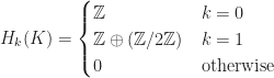
This post will be a guide on how to calculate Homology Groups, focusing on the example of the Klein Bottle. Homology groups can be quite difficult to grasp (it took me quite a while to understand it). Hope this post will help readers to get the idea of Homology. Our reference book will be Hatcher’s Algebraic Topology (Chapter 2: Homology). I will elaborate further on the Hatcher’s excellent exposition on Homology.
This is also Exercise 5 in Chapter 2, Section 2.1 of Hatcher.
The first step to compute Homology Groups is to construct a 

One thing to note for
The key formula for Homology is: 
We have 

Next, we have 

Therefore 
Next, we have 


We then have 


Thus 
To intuitively understand the above working, we need to use the idea that elements in the quotient are “zero”. Hence 


Finally we note that 


In conclusion, we have
Let 


Proof: The trick is to use the Mean Value Theorem for 1 dimension via the following construction:
Define ![g:[0,1]\to\mathbb{R}](https://s0.wp.com/latex.php?latex=g%3A%5B0%2C1%5D%5Cto%5Cmathbb%7BR%7D&bg=ffffff&fg=1a1a1a&s=0&c=20201002)


Let 

This is a basic example of a function of bounded variation on [0,1] but not continuous on [0,1].
The key Theorem regarding functions of bounded variation is Jordan’s Theorem: A function is of bounded variation on the closed bounded interval [a,b] iff it is the difference of two increasing functions on [a,b].
Consider
Both 

URL: https://career-test.com/s/sgamb?reid=210
The results of this Personality Test is quite surprisingly accurate, do give it a try to see if you are a Careerist, Entrepreneur, Harmonizer, Idealist, Hunter, Internationalist or Leader?
Do try out this Free Career Guidance Personality Test at https://career-test.com/s/sgamb?reid=210 while it is still available!
Benefits of doing the (Free) Career Test:
Bought a Mud Crab from Sheng Shiong at $6. The live ones were even cheaper, at $4 each. Much cheaper than ordering crab outside at restaurants, where they would at least cost $30.
My wife then cooked the crab in the “Chilli Crab” style. Yummy!


Just to compile a list of Fundamental groups, Homology Groups, and Covering Spaces for common spaces like the Circle, n-sphere (

Circle:
n-Sphere: 
n-Torus: 

Real projective plane:
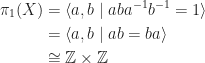
Klein bottle

Klein bottle,
A universal cover of a connected topological space 


Question: Prove that every non-empty open set in
The key things to prove are the disjointness and the countability of such open intervals. Otherwise, if disjointness and countability are not required, we may simply take a small open interval centered at each point in the open set, and their union will be the open set.
Elementary Proof: Let
Let 


We note that such maximal intervals are equal or disjoint: Suppose 


Each of the maximal open intervals contain a rational number, thus we may write 
There are many other good proofs of this found here (http://math.stackexchange.com/questions/318299/any-open-subset-of-bbb-r-is-a-at-most-countable-union-of-disjoint-open-interv), though some can be quite deep for this simple result.

(See more at: http://www.lifehack.org/articles/lifestyle/7-cardinal-rules-life-everyone-should-know-about.html)
Something interesting I realised in my studies in Math is that certain theorems are more “useful” than others. Certain theorems’ sole purpose seem to be an intermediate step to prove another theorem and are never used again. Other theorems seem to be so useful and their usage is everywhere.
One of the most “useful” theorems in basic Ring theory is the following:
Let
(i) 
(ii)
With this theorem, the following question is solved effortlessly:
Let 

(i) Show that 
(ii) Show that
Sketch of Proof of (i):


(ii) is proved similarly.
Just to share a very inspiring motivational video from YouTube. Not sure which movie it is from. (any readers know, please comment below as I would be interested)
Highly suitable for students (and their parents) who have just completed their PSLE, whether their PSLE 2015 results are good or not, it is now a good time to reflect on their dreams and the next step to take in the next year 2016.
There are various methods of computing fundamental groups, for example one method using maximal trees of a simplicial complex (considered a slow method). There is one “trick” using van Kampen’s Theorem that makes it relatively fast to compute the fundamental group.
This “trick” doesn’t seem to be explicitly written in books, I had to search online to learn about it.
First we let


Then, by Seifert-van Kampen Theorem, 


Let 

Therefore

Question: Let 


There is a pretty neat trick to do this question, known as the “interpolation technique”. The proof is as follows.
For 


Thus
Note that the magical thing about the interpolation technique is that 


Finally, the LaTeX path not specified problem has been solved by WordPress!
This post is about how to prove that 
A tempting thing to do is to use the “Second Isomorphism Theorem”, 

The correct way is to note that 
Therefore 

Therefore 


Thus, we have 
Recently, there is a “latex path not specified” WordPress LaTeX bug, it is very weird. Some LaTeX expressions will get rendered and some will not. Will have to postpone my math blogging till it is fixed. Worst case scenario is I have to abandon this blog and move to Blogger (http://mathtuition88.blogspot.com) if the issue remains unfixed.
Testing: 


Hope this bug gets fixed soon. If anyone knows the solution to solve this bug, please inform me in the comments below!
Note: Thanks to Professor Terence Tao who has replied in the comments below and shown us a link where there is ongoing discussion about the highly mysterious “latex path not specified” issue.
Let 


Solution:
The solution strategy is to use simple functions (common tactic for measure theory questions).
Let 

Consider the set 

Then,
Sincere thanks to readers who have completed the Free Personality Quiz!
Today we will revise some basic Group Theory. Let 


Answer: 

Proof:
Our strategy is to prove that 

Now, we have 

Suppose to the contrary there exists 

Since 


Thus 

Instead of committing to regular tuition sessions throughout the year, some students who need academic help are choosing to attend such classes on an “ad-hoc” basis.. Read more at straitstimes.com.
Just heard from a reliable source (cousin who is in the school) that SAJC’s tentative retention rate for 2015 is around 10%. On average, for a class of 25, around 2 or 3 are retained, after the Promos (Promotional Exams) in JC 1.
This is an estimate, intended to give information to those seeking it, hope it helps. By today’ s standards, 10% retention rate is considered “moderate”, considering official statistics from MOE shows that “The two JCs with the highest retention rates at JC1 averaged around 15% over the past three years.”
Side note: Some of those “retained” in SAJC are given a second chance to take another exam, upon passing they can be promoted. Hence the actual retain rate will be less than 10%, which is considered quite ok (compared to other JCs).
Success consists of going from failure to failure without loss of enthusiasm.
For those who are retained, do not despair, check out my motivational page for motivational quotes and stories.
Actually JC life is difficult for students, they have to wake up at 6am everyday, and go home at around 6-7 pm or later (due to CCA). After reaching home, it is just the beginning and they have to revise / do homework / go for tuition. It is much tougher than even the typical adult’s job of 8-5pm work. And JC students have to repeat the schedule daily for two years. The problem is that too much stuff is being crammed into two years.
Apparently, the retain rate / retention rate of JCs is a source of concern for many. Some official statistics has been released by MOE. The statistics given are “over the last three years, approximately 6% of first year JC students in each cohort failed some subjects in their promotional exams and were retained.” “The two JCs with the highest retention rates at JC1 averaged around 15% over the past three years.”
As a student who has gone through the system, rumours of JCs like MJC having 50% retain rate (most likely exaggerated, but having some basis of truth, since there is no smoke without fire) do cause some concern. Currently the JC system works by setting extremely tough internal exams, including promos and prelims (compared to the A levels), such that a D or E in the prelims in top JCs (e.g. RI/HCI/NJC) is very likely equivalent to an A in the eventual A levels. This works for some students to spur them to study harder, but may be overly demoralising for many students. For retention rate, common sense and logic would tell that a high retention rate would boost the school’s eventual A level results (one extra year of study is a lot), however that is at the expense of the student spending one extra year in JC. Since the retention rate is entirely up to the school’s decision (i.e. not regulated by MOE), each JC has different retain rate.
Students choosing a JC should check out their retention rate from reliable seniors / relatives / teachers (there is no official source released online for individual retention rate for JCs).
For students looking for tuition, do check out a highly recommended tuition agency.
Just watched this again. I can truely say that this is the most clear explanation of Homology on the entire internet!
This video follows after the previous video on Simplicial Complexes.
If you are looking for quality Math textbooks to study from (including Linear Algebra and Calculus, the two most popular Math courses), check out my page on Recommended Math Books for students!
Just to share some motivational quotes and stories, including those that are relevant to life, education and math. Do also check out Motivational Books for the Student (Educational).
If you have any other quotes / stories that you like, do post it in the comments! 🙂
1) “Success consists of going from failure to failure without loss of enthusiasm.”
This applies especially to students in higher education (e.g. Junior Colleges in Singapore), where it is quite common to “fail” an exam by getting below 50%. Do not despair, and continue to study hard, and you will achieve success eventually.
2)
“There is nothing noble in being superior to your fellow man; true nobility is being superior to your former self.”
― Ernest Hemingway
Do not compare yourself with your classmates, everyone is unique. Focus on improving yourself day by day.
3)
Kirby tried his qualifying exam again, on the same two topics. “This time, they said, ‘You passed,’” he says. “They didn’t say it with any enthusiasm, but they said, ‘You passed.’” His committee recommended that Kirby move into some other field than topology.
But Kirby was not one to be deterred by discouragement from his teachers. He waited until their backs were turned, so to speak, and identified a topologist — Eldon Dyer — who had been away when Kirby took his qualifying exam. Kirby kept going to Dyer with questions, and “at some point it sort of became obvious that I was his student,” Kirby says. “And he told somebody later on that he realized at some point or other he was stuck with me.”
(https://www.simonsfoundation.org/science_lives_video/robion-kirby/)
Inspirational story from Rob Kirby (famous mathematician) on how to ignore discouragement, even from teachers. This is applicable to students in Singapore who are sometimes told by teachers / school to drop certain subjects (e.g. drop Higher Chinese / drop A Maths), where the motive may not be purely in the student’s interest. Sometimes the reason that the school wants the student to drop the subject is to protect the school’s ranking in the exams / boost principal’s KPI etc. In this case, the student should follow his own judgement on whether to drop the subject.
4)
“Everyone is No. 1” Motivational Song by Andy Lau.
Beautiful Lyrics (Chinese):
我的路不是你的路
我的苦不是你的苦
每个人都有潜在的能力
把一切去征服
我的泪不是你的泪
我的痛不是你的痛
一样的天空不同的光荣
有一样的感动
不需要自怨自艾的惶恐
只需要沉着
只要向前冲
告诉自己天生我才必有用
Everyone is NO.1
只要你凡事不问能不能
用一口气交换你一生
要迎接未来不必等
Everyone is NO.1
成功的秘诀在你肯不肯
流最热的汗
拥最真的心
第一名属于每个人
我的手不是你的手
我的口不是你的口
只要一条心
暴风和暴雨
都变成好朋友
不需要自怨自艾的惶恐
只需要沉着
只要向前冲
告诉自己天生我才必有用
不害怕路上有多冷
直到还有一点余温
我也会努力狂奔
Everyone is NO.1
只要你凡事不问能不能
用一口气交换你一生
要迎接未来不必等
Everyone is NO.1
成功的秘诀在你肯不肯
流最热的汗
拥最真的心
第一名属于每个人
5)
Success is not final, failure is not fatal: it is the courage to continue that counts.
6)
Galatians 6:4-6Easy-to-Read Version (ERV)
4 Don’t compare yourself with others. Just look at your own work to see if you have done anything to be proud of. 5 You must each accept the responsibilities that are yours.
Try out the Personality Quiz!
This inequality often appears in Analysis: 


It turns out that the key is to use convexity, and we can even prove a stronger version of the above, namely 
Proof: Consider 

Choose 


Thus,
Click here for Free Personality Test
Question: What is 

Algebraically, the dihedral group may be viewed as a group with two generators 


Answer:

For
Proof: For 


For 

Let 

Let 


I.e. the only element in 
Let 

By earlier analysis, this is true iff 


Therefore,
For
Just heard from some sources that AJC (Anderson Junior College) Math papers are considered the most difficult of all JCs, beating RI/HCI in terms of difficulty.
Do check out this page on how to calculate JC Ranking points.
Quotes:
AJC might have the most challenging Math papers, but that doesn’t equate to having the best math results. Other schools do better (RI/HCI)
From: http://forums.sgclub.com/singapore/ajc_good_jc_386546.html
H2 Maths this year was quite easy for both paper 1 & 2. It is definitely no where of the standard of AJC Maths Exam Papers, which are famously known for very challenging questions.
From: http://doggy94-in-air.blogspot.sg/
WordAds 2.0 is out. Hope it is good news for international WordPress blogs, who are getting much lower ad revenue compared to the US and Europe.
Today, we’re excited to introduce you to a new WordAds. On the front end, it’s a simpler and more streamlined experience like never before. On the back-end we have launched a real-time bidding platform to maximize earnings and ad creative control. Say hello to WordAds 2.0!
WordAds 2.0 is now fully integrated where you control the rest of your blog, in WordPress.com’s main Settings interface. You can also view your Earnings reports here and manage your payout information.

Existing WordAds users aren’t the only ones to benefit from the changes in WordAds 2.0. For new users, we have done away with the separate application process. Any family friendly WordPress.com blog with minimal page views will be considered for immediate admission to WordAds.
Bigger changes are now live in our real time bidding environment. We have dozens of ad agencies and buyers bidding in real time on each of our global…
View original post 92 more words
The above video describes the real projective plane (
The projective space 


Notation: For 
![[x_1, x_2,\dots, x_{n+1}]](https://s0.wp.com/latex.php?latex=%5Bx_1%2C+x_2%2C%5Cdots%2C+x_%7Bn%2B1%7D%5D&bg=ffffff&fg=1a1a1a&s=0&c=20201002)

![f[x,y]=[x,y,0]](https://s0.wp.com/latex.php?latex=f%5Bx%2Cy%5D%3D%5Bx%2Cy%2C0%5D&bg=ffffff&fg=1a1a1a&s=0&c=20201002)
![g[x,y]=[x,-y,0]](https://s0.wp.com/latex.php?latex=g%5Bx%2Cy%5D%3D%5Bx%2C-y%2C0%5D&bg=ffffff&fg=1a1a1a&s=0&c=20201002)
How do we construct an explicit homotopy between ![F([x,y],t)=[x,(1-2t)y,0]](https://s0.wp.com/latex.php?latex=F%28%5Bx%2Cy%5D%2Ct%29%3D%5Bx%2C%281-2t%29y%2C0%5D&bg=ffffff&fg=1a1a1a&s=0&c=20201002)
A better approach is to consider 
![\boxed{F([x,y],t)=[x,(\cos\pi t)y, (\sin\pi t)y]}](https://s0.wp.com/latex.php?latex=%5Cboxed%7BF%28%5Bx%2Cy%5D%2Ct%29%3D%5Bx%2C%28%5Ccos%5Cpi+t%29y%2C+%28%5Csin%5Cpi+t%29y%5D%7D&bg=ffffff&fg=1a1a1a&s=0&c=20201002)
Note that if 
![x^2+[(\cos\pi t)y]^2+[(\sin\pi t)y]^2=x^2+y^2=1](https://s0.wp.com/latex.php?latex=x%5E2%2B%5B%28%5Ccos%5Cpi+t%29y%5D%5E2%2B%5B%28%5Csin%5Cpi+t%29y%5D%5E2%3Dx%5E2%2By%5E2%3D1&bg=ffffff&fg=1a1a1a&s=0&c=20201002)

Just to share this news:
The National Taiwan University is holding the first ever Calculus World Cup (CWC) in February 2016. It’s the first time students from global top universities will be able to compete over Calculus in e-sports. The competition will be held on PaGamO – a social online gaming platform for education. The top 12 teams will be invited to Taiwan for the final round, and great prizes with a value of over $70,000 await the finalists!
Official website: http://cwc.pagamo.com.tw
Registration: https://pagamo.com.tw/calculus_cup
Facebook: https://www.facebook.com/PaGamo.glo
Click here for: Free Personality Quiz
Recall that a space Y is contractible if the identity map 


Proof: Let Y be a contractible space and let X be any space. 
![F: Y\times [0,1]\to Y](https://s0.wp.com/latex.php?latex=F%3A+Y%5Ctimes+%5B0%2C1%5D%5Cto+Y&bg=ffffff&fg=1a1a1a&s=0&c=20201002)


Let ![G:X\times [0,1]\to Y](https://s0.wp.com/latex.php?latex=G%3AX%5Ctimes+%5B0%2C1%5D%5Cto+Y&bg=ffffff&fg=1a1a1a&s=0&c=20201002)
When 


Therefore
Just chanced upon this video on YouTube, really made a lot of sense and is very uplifting. Dream big, and don’t set any limits on yourself and what you can do.
Some other books by Nick:
Free Career Quiz: Please help to do!
Just came across this neat beginner’s Lebesgue Theory question. As students of analysis know, just to show a set is measurable is no easy feat. The usual way is to use the Caratheodory definition, where a set E is said to be measurable if for any set A, 
Question: Suppose E is a Lebesgue measurable set and let F be any subset of 
The short way to do this is to note that 


Next comes the critical observation: 

Thus 
Interesting indeed!
Click here for free Career Quiz: https://career-test.com/s/sgamb?reid=210
I came across this joke on another blog: http://phdlife.warwick.ac.uk/
Quite true! A Math student will understand this at the university level and beyond, where Math has no more numbers and is full of symbols and jargon! Although even the most abstract Math has applications, the applications are only discovered years later, hence Pure Math is indeed one of the most pure subjects around.


![[G:\ker\sigma]=[G:H][H:\ker\sigma]=p[H:\ker\sigma]](https://s0.wp.com/latex.php?latex=%5BG%3A%5Cker%5Csigma%5D%3D%5BG%3AH%5D%5BH%3A%5Cker%5Csigma%5D%3Dp%5BH%3A%5Cker%5Csigma%5D&bg=ffffff&fg=1a1a1a&s=0&c=20201002)
![p_*([f]):=[pf]](https://s0.wp.com/latex.php?latex=p_%2A%28%5Bf%5D%29%3A%3D%5Bpf%5D&bg=ffffff&fg=1a1a1a&s=0&c=20201002)
![p_*([f]+[g])=[p(f+g)]](https://s0.wp.com/latex.php?latex=p_%2A%28%5Bf%5D%2B%5Bg%5D%29%3D%5Bp%28f%2Bg%29%5D&bg=ffffff&fg=1a1a1a&s=0&c=20201002)
![p(f+g)(s_1,s_2,\dots,s_n)=\begin{cases}pf(2s_1,s_2,\dots,s_n)&s_1\in[0,\frac 12]\\ pg(2s_1-1,s_2,\dots,s_n)&s_1\in[\frac 12,1] \end{cases}](https://s0.wp.com/latex.php?latex=p%28f%2Bg%29%28s_1%2Cs_2%2C%5Cdots%2Cs_n%29%3D%5Cbegin%7Bcases%7Dpf%282s_1%2Cs_2%2C%5Cdots%2Cs_n%29%26s_1%5Cin%5B0%2C%5Cfrac+12%5D%5C%5C++++pg%282s_1-1%2Cs_2%2C%5Cdots%2Cs_n%29%26s_1%5Cin%5B%5Cfrac+12%2C1%5D++++%5Cend%7Bcases%7D&bg=ffffff&fg=1a1a1a&s=0&c=20201002)
![p_*[f]+p_*[g]=[pf]+[pg]](https://s0.wp.com/latex.php?latex=p_%2A%5Bf%5D%2Bp_%2A%5Bg%5D%3D%5Bpf%5D%2B%5Bpg%5D&bg=ffffff&fg=1a1a1a&s=0&c=20201002)


![F([x,y],0)=[x,y,0]](https://s0.wp.com/latex.php?latex=F%28%5Bx%2Cy%5D%2C0%29%3D%5Bx%2Cy%2C0%5D&bg=ffffff&fg=1a1a1a&s=0&c=20201002)
![F([x,y],1)=[x,-y,0]](https://s0.wp.com/latex.php?latex=F%28%5Bx%2Cy%5D%2C1%29%3D%5Bx%2C-y%2C0%5D&bg=ffffff&fg=1a1a1a&s=0&c=20201002)


