Complex Integrals

According to Churchill’s book Complex Variables and Applications,

Integrals are extremely important in the study of functions of a complex variable. The theory of integration, to be developed in this chapter, is noted for its mathematical elegance. The theorems are generally concise and powerful, and many of the proofs are short.

Basic Contour Integrals

The basic way of computing contour integrals is to use the definition. There are more advanced and very powerful methods of computing contour integrals, which we will mention in later posts.

The summarised definition is as follows: $\int_C f(z)\ dz=\int_a^b f[z(t)]z'(t)\,dt$ where $z=z(t), a\leq t\leq b$ represents a contour $C$ .

Basic Example 1: $I=\int_C \bar{z}\,dz$ , where $C$ is the contour $z=2e^{i\theta}$ , $-\pi/2\leq\theta\leq\pi/2$ .

Using the definition, we have

$\begin{aligned} I&=\int_{-\pi/2}^{\pi/2}2e^{-it}\cdot 2ie^{it}\,dt\\ &=4i\int_{-\pi/2}^{\pi/2} 1\,dt\\ &=4\pi i \end{aligned}$

Let $(A,+,\mu)$ be an $R$ -algebra. Define an operation $\mu': A\times A\to A$ by $\mu'(a,b)=\mu(b,a)=ba$ . This algebra $(A,+,\mu')$ is called the opposite algebra to $A$ . We verify that it forms an $R$ -algebra.

Bilinearity comes from the following computations:

$\mu'(a_1+a_2,b)=b(a_1+a_2)=ba_1+ba_2=\mu'(a_1,b)+\mu'(a_2,b)$

$\mu'(a,b_1+b_2)=(b_1+b_2)a=b_1a+b_2a=\mu'(a,b_1)+\mu'(a,b_2)$

$\mu'(ar,b)=bar=\mu'(a,b)r$

$\mu'(a,br)=bra=bar=\mu'(a,b)r$

Associativity is true from $\mu'(\mu'(a,b),c)=cba=\mu'(a,\mu'(b,c))$

The unity element is the same unity element $1_A$ : $\mu'(x,1_A)=1_Ax=x$ , $\mu'(1_A,x)=x1_A=x$ .

Center of Matrix Algebra / Matrix Ring is Scalar Matrices

We will prove that the center $Z(M_n(A))=Z(A)I_n$ , where $A$ is an $R$ -algebra (or ring with unity).

One direction is pretty clear. Let $X\in Z(A)I_n, Y\in M_n(A)$ . Then $X=zI_n$ for some $z\in Z(A)$ . $XY=zI_n Y=zY$ , $YX=YzI_n=zY$ , so $X$ is in the center $Z(M_n(A))$ .

The other direction will require the use of $E_{ij}$ matrices, which is a n by n matrix with (i,j) entry 1, and rest zero.

Let $X=(x_{ij})\in Z(M_n(A))$ . We can write $X=\sum x_{ij}E_{ij}$ . Our key step is compute $E_{pq}X=\sum x_{qj}E_{pj}=XE_{pq}=\sum x_{ip}E_{iq}$ . Thus we may conclude that

$(E_{pq}X)_{ij}=\begin{cases}x_{qj}&\text{if}\ i=p\\ 0&\text{otherwise} \end{cases}$

$(XE_{pq})_{ij}=\begin{cases}x_{ip}&\text{if}\ j=q\\ 0&\text{otherwise} \end{cases}$

Plugging in some convenient values like $i=p, j=q$ , we can conclude that $x_{qq}=x_{pp}$ for all $p,q$ , i.e. all diagonal entries are equal.

Plug in $i=p, j\neq q$ gives us $x_{qj}=0$ for all $j\neq q$ .

Thus $X$ is a scalar matrix, i.e. $X=\alpha I_n$ for some $\alpha\in A$ .

Observing that $(\beta I_n)X=\beta\alpha I_n=X(\beta I_n)=\alpha\beta I_n$ , we conclude that $\beta\alpha=\alpha\beta$ for all $\beta$ in $A$ . So $\alpha$ has to be in the center $Z(A)$ .

Gauge (Minkowski functional) of Convex Set

Theorem: Let $K$ be a convex set.

(i) $p_K(x)\leq 1$ if $x\in K$ .

(ii) $p_K(x)<1$ if and only if $x$ is an interior point of $K$ .

We need the following definition: $p_K(x)=\inf\{a\mid a>0,x/a\in K\}$ . This $p_K$ is often known as a Gauge or Minkowski functional.

Proof:

(i) If $x\in K$ , then $x/1\in K$ , so $P_K(x)\leq 1$ . This is the easy part. The converse holds here, if $x\notin K$ , then $p_K(x)>1$ .

(ii) We first prove the “only if” part. Assume $p_K(x)<1$ . Suppose $x$ is not an interior point of $K$ , i.e. there exists $y\in X$ such that for all $\epsilon>0$ , $x+ty\notin K$ for some $|t|<\epsilon$ .

We then have $p_K(x+ty)>1$ . Combining with the subadditive property of the gauge, we have $1<p_K(x+ty)\leq p_K(x)+p_K(ty)$ . Rearranging, we get $p_K(x)>1-p_K(ty)$ . By considering the various possibilities of the sign of $t$ , and using the positive homogeneity of the gauge, we can obtain a contradiction. For example, if $t>0$ , $p_K(x)>1-tp_K(y)$ . Since $t\to 0$ as $\epsilon\to 0$ , this implies $p_K(x)\geq 1$ , a contradiction.

Conversely, if $x$ is an interior point of $K$ , for all $y$ there exists $\epsilon>0$ such that $x+ty\in K$ for all $|t|<\epsilon$ .

We have $p_K(x+ty)\leq 1$ for all $y$ , for all $|t|<\epsilon$ . Since it is a “for all” quantifier, we can choose in particular $y=x$ , $t>0$ .

Then we have $p_K((1+t)x)\leq 1$ , which leads to $(1+t)p_K(x)\leq 1$ and $p_K(x)\leq \frac{1}{1+t}<1$ .

议论文论据素材的积累 Where to Collect Material for Argumentative Composition

Chinese Tuition Singapore

议论文中的论据是用来证明论点的理由和根据。主要有事实论据和道理论据。

一般可以用来作为论据的有很多，如名人名言，俗语谚语，名人轶事，甚至广告词，歌词，身边的事情都可以作为论据。

写作素材的积累需要学生增加阅读量，无论是课外书（小说，诗歌，散文），或是报纸，或者杂志，甚至看一些中文电视节目，这些都是积累的途径。读书破万卷，下笔如有神，读的多了，写文章自然会变成一件容易的事情。

读报纸，可以阅读一些社会热点，并且学习记者在报道新闻和评论新闻的思维，这对口试也是有帮助的。尤其是中学的口试需要对一些社会时事发表自己的观点，多看这类报章，会帮助学生开拓思维。在口试的时候，才会知道该怎么回答，从哪些方面来回答。

看中文电视节目，对学生的作文和口试都有帮助。推荐一档中国的电视节目：

「百家讲坛」这档中国CCTV的科教节目涉及人文科学，自然科学，哲学等。通过看这档节目可以学到很多中国历史典故和国学常识，而且很多名家讲课的内容非常有趣生动。当我还是高中生的时候，课间休息时间，全班学生经常一起看这个节目。比较著名的是（王立群读史记，易中天品三国，于丹论语心得，刘心武揭秘红楼梦，孔庆东看武侠小说，纪连海说清朝二十四臣，等）这些主讲嘉宾，既有著名大学教授，也有作家，还有高中教师。如果对中国文化，历史，文学感兴趣，这是一个很好的节目。

当然如果学生不适合这类比较深的节目，可以尝试一些比较轻松综艺性节目，比如说中国最近有一档节目叫「世界青年说」，这个节目邀请了十多个国家的青年代表（他们来自美，德，英，意，澳等国家），他们每一期节目都会围绕一个议题展开讨论。有一些议题和学生的口试题目非常接近，比如养老，环保，文化差异等等。虽然这些青年代表都是外国人，可是他们的中文水平都不错，对当下中国的流行文化也非常了解。他们在讨论的过程中，会涉及到大量的不同国家的文化风俗，会给观众科普很多典故及历史，这些都是很好的写作素材。而且在他们讨论的过程中也是可以学习他们对某一问题如何发表看法，并且如何论证自己的观点。因为嘉宾都是来自不同的国家和地区，所以在讨论过程中会产生思维碰撞，也可以打开学生的思维，让他们学会从不同的角度去看待同一个问题。

很多家长对成语情有独钟。一些家长会明确要求我给他们的孩子多教成语。我比较推荐学生通过读成语故事的方式来学习成语。因为成语故事本身要么是史实典故，要么是传说，无论是哪种，都是社会普遍认同的，所以故事来当论据是很有分量的。写成语故事还有一个好处，就是凑字数。有些学生会为自己写的作文字数太少而头疼不已。成语故事肯定比只是成语单单这几个字要长的多。

很多学生不喜欢读中文读物，也不喜欢看中文电视节目怎么办？

这种情况下，课本和阅读理解以及阅读问答也可以转变成素材的来源。其实课文中就有很多成语，俗语等。而且课文的写作思路也可以成为借鉴的材料。比如中三的课本中有”老吾老以及人之老””少年莫笑白头翁，人人都有夕阳红””百善孝为先”等可以积累的名语。所以不爱读课外读物的学生，可以把课文内容掌握好，这也算一种方法。

除了课本之外，学生往往也会忽视阅读题目的另外一个作用，就是它也可以当作写作素材。很多阅读题目会选一些名人故事当作材料，这些故事都可以作为论据，而且一个故事可以多用。比如说，有一个理解问答是关于爱因斯坦的。爱因斯坦发表了”相对论”，瑞典皇家科学院很多评委凭借这个理论提名爱因斯坦诺贝尔奖。但是有一个评委反对，因为”相对论”没有经过验证。所以爱因斯坦就没能得到诺贝尔奖。之后一次又一次，爱因斯坦被提名，却被这个评委用同样的借口拒绝。后来有一个叫奥森的年轻人，用”光电效应理论”提名爱因斯坦。这次爱因斯坦终于拿到诺贝尔奖。这个故事涉及到三个人物，而这三个人物刚好是理解这个故事的三个角度。爱因斯坦是著名的科学家，而他拿诺贝尔奖之路漫长又坎坷。开始虽然一次又一次失败，但是他也没有因此沮丧或者气馁，最终他还是拿到了诺贝尔奖，虽然不是凭借”相对论”。从爱因斯坦这个角度，至少可以提炼出两个论点：1，遇到挫折，困难，不可以放弃，要坚持。2，上帝在关闭一扇门的同时，也会打开一扇窗。天无绝人之路。如果从奥森这个角度来讲，也可以提炼出一个论点：换个角度看问题，或者遇事要灵活。如果从投反对票的评委来讲可以从两个方面进行分析：1，坚持原则，刚正不阿，不会因为舆论导向而放弃自己的准则。2，墨守成规，做事呆板，才导致没能给”相对论”应有的荣耀。

所以同一个故事可以从不同的方面去解读，那么学生再遇到与此有关的作文题目，无论是关于坚持，不放弃，又或者换个角度看问题等主题，都可以用这同一个故事当作论据。学生在平时做阅读题目时，要做个有心人。遇到一些名句俗语，或者有深刻含义的故事，都可以记在心里。说不定写作文的时候会派上用场！

View original post

Mapping of Infinite Vertical Strip by the Exponential Function

This post is continued from a previous post on how to map an open region between two circles to a vertical strip. We wish to map the infinite vertical strip $0<\text{Re}(z)<1$ onto the upper half plane. Reference book is Complex Variables and Applications, Example 3 page 44.

First, we need to map the vertical strip onto the horizontal strip $0<y<\pi$ . This is easily accomplished by $w=\pi iz$ . The factor $i$ is responsible for the rotation (90 degree anticlockwise), while the factor $\pi$ is responsible for the scaling.

Let us consider the exponential mapping $w=e^z=e^{x+iy}=e^x\cdot e^{iy}$ . Consider line $y=k$ . This line will be mapped onto the ray (from the origin) with argument $k$ . Since $0<y<\pi$ , the image is a collection of rays of arguments $0<\theta<\pi$ that “sweeps” across and covers the entire upper half plane.

In conclusion, the map $f(z)=e^{\pi i z}$ will do the job for mapping the vertical strip $0<x<1$ onto the upper half plane $y>0$ .

Let A be a simple R-algebra, then M_n(A) is simple

We let $A$ be a simple $R$ -algebra. Then $M_n(A)$ , the n by n matrix algebra over $A$ is simple. In particular if $D$ is a division algebra, then $M_n(D)$ is simple.

Reference: Associative Algebras (Graduate Texts in Mathematics)

We will split our proof into 2 Lemmas.

Lemma 1: If $I\lhd A$ , then $M_n(I)\lhd M_n(A)$ .

Proof: Let $X=(x_{ij}), Y=(y_{ij})\in M_n(I), Z=(z_{ij})\in M_n(A)$ .

$(X-Y)_{ij}=x_{ij}-y_{ij}\in I$ . Therefore $X-Y\in M_n(I)$ .

$(XY)_{ij}=\sum_{k=1}^n x_{ik}y_{kj}\in I$ , thus $XY\in M_n(I)$ . Similarly $YX\in M_n(I)$ . Thus $M_n(I)$ is indeed an ideal of $M_n(A)$ .

Lemma 2 (Tricky part, takes some time to digest): If $J\lhd M_n(A)$ , then $J=M_n(I)$ for some $I\lhd A$ .

A technical thing we need to know is the $E_{ij}$ matrix, which is a n by n matrix with 1 in the (i,j) entry, 0 elsewhere. A key property is that $E_{ij}E_{kl}=E_{il}$ if $j=k$ , and 0 otherwise (zero matrix).

The key idea here is that $I$ can be taken to be $I=\{r\in A\mid rE_{11}\in J\}$ . We can check that $I$ is indeed an ideal. We need to know that it is possible to premultiply and postmultiply a given matrix by “elementary matrices” such that any entry of the given matrix is “shifted” to the (1,1) entry. An example will be $\begin{pmatrix}0&1\\0&0\end{pmatrix}\begin{pmatrix}a&b\\c&d\end{pmatrix}\begin{pmatrix}0&0\\1&0\end{pmatrix}=\begin{pmatrix}d&0\\0&0\end{pmatrix}$ .

Let us begin the proof to first show $J\subseteq M_n(I)$ . Let $X=(x_{ij})\in J$ . We write $X=\sum_{i,j}^n x_{ij}E_{ij}$ . For any $1\leq p,q\leq n$ ,

$\begin{aligned}E_{1p}XE_{q1}&=E_{1p}(\sum x_{ij}E_{ij})E_{q1}\\ &=(\sum x_{pj}E_{1j})E_{q1}\\ &=x_{pq}E_{11}\in J \end{aligned}$

Therefore $x_{pq}\in I$ . Therefore $X\in M_n(I)$ . What we are actually doing here is first pick an arbitrary matrix $X$ in $J$ . Then, we do the “shifting” process to show that any (p,q) entry in $X$ can be “shifted” to the (1,1) entry, thus it is inside our ideal $I$ . Since any arbitrary (p,q) entry in $X$ is inside the ideal $I$ , we conclude that $X$ is an element of $M_n(I)$ .

Next part is to show $M_n(I)\subseteq J$ . Let $X=(x_{ij})\in M_n(I)$ . We have $x_{ij}E_{11}\in J$ for all $i,j$ . We compute that

$\begin{aligned}E_{i1}(x_{ij}E_{11})E_{1j}&=x_{ij}E_{i1}E_{1j}\\ &=x_{ij}E_{ij}\in J \end{aligned}$

Therefore $X=\sum x_{ij}E_{ij}\in J$ . We will illustrate what we are doing here by an example in the 2 by 2 case. Let us have $X=\begin{pmatrix}a&b\\c&d\end{pmatrix}$ . Since $X$ is in $M_n(I)$ , what we have, by definition of $I$ , is that $\begin{pmatrix}a&0\\0&0\end{pmatrix}$ , $\begin{pmatrix}b&0\\0&0\end{pmatrix}$ , $\begin{pmatrix}c&0\\0&0\end{pmatrix}$ , $\begin{pmatrix}d&0\\0&0\end{pmatrix}$ are all in $J$ . We then proceed to “shift” them all into their correct positions: $\begin{pmatrix}a&0\\0&0\end{pmatrix}$ , $\begin{pmatrix}0&b\\0&0\end{pmatrix}$ , $\begin{pmatrix}0&0\\c&0\end{pmatrix}$ , $\begin{pmatrix}0&0\\0&d\end{pmatrix}$ , all of which are still in the ideal $J$ . $X$ is the sum of all of them, thus also in $J$ .

Final Conclusion

Since $A$ is simple, its ideals are 0 and itself. Thus, the ideals of $M_n(A)$ will be also the 0 matrix and itself, and thus is simple. A division algebra $D$ is simple (Any ideal containing a nonzero element $x$ , when multiplied by its inverse will give 1. Thus the ideal will contain 1 and thus the entire ring $D$ ), thus $M_n(D)$ is also simple.

Ultimate Tic-Tac-Toe

Math with Bad Drawings

Updated 7/16/2013 – See Original Here

Once at a picnic, I saw mathematicians crowding around the last game I would have expected: Tic-tac-toe.

As you may have discovered yourself, tic-tac-toe is terminally dull. There’s no room for creativity or insight. Good players always tie. Games inevitably go something like this:

But the mathematicians at the picnic played a more sophisticated version. In each square of their tic-tac-toe board, they’d drawn a smaller board:

As I watched, the basic rules emerged quickly.

View original post 434 more words

Image of Infinite Strip under Transformation w=1/z

Q: Find the image of the infinite strip $0<y<1/(2c)$ under the transformation $w=1/z$ .

(This question is taken from Complex Variables and Applications (Brown and Churchill))

Answer: $u^2+(v+c)^2>c^2$ , $v<0$ .

Solution:

We are using the standard notation $w=u+iv$ , $z=x+iy$ . From the equation $\displaystyle z=\frac{1}{w}=\frac{1}{u+iv}=\frac{u-iv}{u^2+v^2}$ , we can conclude that $\displaystyle y=\frac{-v}{u^2+v^2}$ .

With some algebra and completing the square, one can obtain $u^2+(v+\frac{1}{2y})^2=(\frac{1}{2y})^2$ , which is the equation of a circle centered at $(0,-\frac{1}{2y})$ with radius $1/2y$ . When $y=1/(2c)$ , the equation of the circle is $u^2+(v+c)^2=c^2$ . As $y$ gets smaller (closer to zero), the radius of the circle becomes larger, while still remaining tangent to the horizontal axis.

Thus, the image of the strip is $u^2+(v+c)^2>c^2$ , $v<0$ .

Analytic Isomorphism (Complex Analysis)

An analytic isomorphism $f:U\to V$ (where $U$ and $V$ are open sets) is an analytic function such that there exists another analytic function $g:V\to U$ , satisfying $f\circ g=id_V$ and $g\circ f=id_U$ .

(1/2)! = (√π)/2

Math Online Tom Circle

Richard Feynman (Nobel Physicist) proved it in high school using a funny Calculus: “Differentiating under Integral” — is it legitimate to do so ? Of course it is by “The Fundamental Theorem of Calculus”

Note: We were thought in high school the “HOW” of calculating (such as integration and differentiation), but not the “WHY” (the Theorem behind). Richard Feynman was unique in exploring the WHY since high school, it helped later he was assigned by President Reagan to investigate the 1986 ‘Challenger’ disaster ?

View original post

Piper Harron discusses her artistic and wonderful math Ph.D. thesis

This is the most “unique” PhD thesis I have ever seen. Very special, and humorous to read, and coming from the most elite institution Princeton, under the guidance of Fields Medalist Manjul Bhargava.

mathbabe

Piper Harron is a mathematician who is very happy to be here, and yes, is having a great time, despite the fact that she is standing alone awkwardly by the food table hoping nobody will talk to her.

Piper, would you care to write a mathbabe post describing your thesis, and yourself, and anything else you’d care to mention?

When Cathy (Cathy? mathbabe?) asked if I would like to write a mathbabe post describing my thesis, and myself, and anything else I’d care to mention, I said “sure!” because that is objectively the right answer. I then immediately plunged into despair.

Describe my thesis? My thesis is this thing that was initially going to be a grenade launched at my ex-prison, for better or for worse, and instead turned into some kind of positive seed bomb where flowers have sprouted beside the foundations I thought I wanted to crumble…

View original post 649 more words

2015 in review

The WordPress.com stats helper monkeys prepared a 2015 annual report for this blog.

Here’s an excerpt:

The Louvre Museum has 8.5 million visitors per year. This blog was viewed about 170,000 times in 2015. If it were an exhibit at the Louvre Museum, it would take about 7 days for that many people to see it.

Click here to see the complete report.

Rouche’s Theorem and Applications

This blog post is on Rouche’s Theorem and some applications, namely counting the number of zeroes in an annulus, and the fundamental theorem of algebra.

Rouche’s Theorem: Let $f(z)$ , $g(z)$ be holomorphic inside and on a simple closed contour $K$ , such that $|g(z)|<|f(z)|$ on $K$ . Then $f$ and $f+g$ have the same number of zeroes (counting multiplicities) inside $K$ .

Rouche’s Theorem is useful for scenarios like this: Determine the number of zeroes, counting multiplicities, of the polynomial $f(z)=2z^5-6z^2-z+1=0$ in the annulus $1\leq |z|\leq 2$ .

Solution:

Let $K_1$ be the unit circle $|z|=1$ . We have

$\begin{aligned}|2z^5-z+1|&\leq |2z^5|+|z|+|1|\\ &=2+1+1\\ &=4\\ &<6\\ &=|-6z^2| \end{aligned}$

on $K_1$ .

Since $-6z^2$ has 2 zeroes in $K_1$ , therefore $f$ has 2 zeroes inside $K_1$ , by Rouche’s Theorem.

Let $K_2$ be the circle $|z|=2$

$\begin{aligned} |-6z^2-z+1|&\leq |-6z^2|+|-z|+|1|\\ &=6(2^2)+2+1\\ &=27\\ &<64\\ &=|2z^5| \end{aligned}$

on $K_2$ . Therefore $f$ has 5 zeroes inside $K_2$ .

Therefore $f$ has 5-2=3 zeroes inside the annulus.

We do a computer check using Wolfram Alpha (http://www.wolframalpha.com/input/?i=2z%5E5-6z%5E2-z%2B1%3D0). The moduli of the five roots are (to 3 significant figures): 0.489, 0.335, 1.46, 1.45, 1.45. This confirms that 3 of the zeroes are in the given annulus.

Fundamental Theorem of Algebra Using Rouche’s Theorem

Rouche’s Theorem provides a rather short proof of the Fundamental Theorem of Algebra: Every degree n polynomial with complex coefficients has exactly n roots, counting multiplicities.

Proof: Let $f(z)=a_0+a_1z+a_2z^2+\dots+a_nz^n$ . Chose $R\gg 1$ sufficiently large so that on the circle $|z|=R$ ,

$\begin{aligned} |a_0+a_1z+a_2z^2+\dots+a_{n-1}z^{n-1}|&\leq|a_0|+|a_1|R+|a_2|R^2+\dots+|a_{n-1}|R^{n-1}\\ &<(\sum_{i=0}^{n-1}|a_i|)R^{n-1}\\ &<|a_n|R^n\\ &=|a_nz^n| \end{aligned}$

Since $a_nz^n$ has $n$ roots inside the circle, $f$ also has $n$ roots in the circle, by Rouche’s Theorem. Since $R$ can be arbitrarily large, this proves the Fundamental Theorem of Algebra.

Culture, Intellect & Attitude

Math Online Tom Circle

Culture, Intellect & Attitude Most Important
Let f: {A,B…Y,Z} -> {1,2… 25,26}
f(AB}=f(A)+f(B)=1+2=3
=> f homomorphism

f(LUCK)= f(L)+f(U)+f(C)+f(K)= 12+21+3+11 =47
f(LOVE)=54
f(KNOWLEDGE)=96
f(LEADERSHIP)=97
f(HARDWORK)=98

f(CULTURE)=100
f(INTELLECT)=100
f(ATTITUDE)=100
=> Last 3 most important in life!

View original post

Galois Group (Example)

This post is about the Galois group of $K$ over $\mathbb{Q}$ , where $K$ is the splitting field of $f(x)=x^p-2$ , where $p$ is an odd prime.

First we show that the polynomial $f(x)=x^p-2$ is irreducible over $\mathbb{Q}$ . This follows immediately by Eisenstein’s Criterion, since $2\mid (-2)$ , $2\nmid 1$ and $2^2\nmid (-2)$ .

Next, we show that the splitting field $K$ of $f(x)$ in $\mathbb{C}$ is $Q(\sqrt[p]{2},\omega)$ , where $\omega=e^{2\pi i/p}$ is a primitive p-th root of unity. The roots of $f$ are $\sqrt[p]2, \sqrt[p]2\omega, \sqrt[p]2\omega^2, \dots, \sqrt[p]2\omega^{p-1}$ .

The splitting field $K$ contains $\sqrt[p]2$ and $\omega=\frac{\sqrt[p]2\omega^2}{\sqrt[p]2\omega}$ . Thus $\mathbb{Q}(\sqrt[p]2,\omega)\subseteq K$ .

On the other hand, $\mathbb{Q}(\sqrt[p]2,\omega)$ contains all the roots of $f$ , hence $f$ splits in $\mathbb{Q}(\sqrt[p]2, \omega)$ . Thus $K\subseteq\mathbb{Q}(\sqrt[p]2,\omega)$ , since $K$ is the smallest field that contains $\mathbb{Q}$ and all the roots of $f$ . All in all, we have that the splitting field $K=\mathbb{Q}(\sqrt[p]2, \omega)$ .

The next part involves determining the Galois group of $K$ over $\mathbb{Q}$ . We have $|Gal(K/\mathbb{Q})|=[K:\mathbb{Q}]$ . Since $[\mathbb{Q}(\sqrt[p]2):\mathbb{Q}]=p$ (minimal polynomial $x^p-2$ ), and $[\mathbb{Q}(\omega):\mathbb{Q}]=p-1$ (minimal polynomial the cyclotomic polynomial $1+x+x^2+\dots+x^{p-1}$ ), thus $|Gal(K/\mathbb{Q})|=p(p-1)$ . Here we have used the lemma that suppose $[F(\alpha):F]=m$ and $[F(\beta):F]=n$ with $\gcd(m,n)=1$ , then $[F(\alpha,\beta):F]=mn$ .

What the Galois group does is it permutes the roots of $f$ . Let $\sigma$ be an element of the Galois group. $\sigma(\sqrt[p]2)$ can possibly be $\sqrt[p]2, \sqrt[p]\omega, \dots, \sqrt[p]2\omega^{p-1}$ , a total of $p$ choices. Similarly, $\sigma(\omega)=\omega, \omega^2, \dots,\omega^{p-1}$ , a total of $p-1$ choices. All these total up to $p(p-1)$ elements, which is exactly the size of the Galois group.

The above Galois group $Gal(K/\mathbb{Q})$ is described by how its elements act on the generators. For a more concrete representation, we can actually prove that the Galois group above is isomorphic to the group of matrices $\begin{pmatrix}a&b\\0&1\end{pmatrix}$ , where $a,b\in\mathbb{F}_p$ , $a\neq 0$ . We denote the group of matrices as $M$ .

To show the isomorphism, we define a map $\phi: Gal(K/\mathbb{Q})\to M$ , mapping $\sigma_{a,b}$ to $\begin{pmatrix}a&b\\0&1\end{pmatrix}$ .

Notation: $\sigma_{a,b}$ is defined on the generators as follows, $\sigma_{a,b}(\sqrt[p]2)=\sqrt[p]2\omega^b$ , $\sigma_{a,b}(\omega)=\omega^a$ .

We can clearly see that the map $\phi$ is bijective. To see it is a homomorphism, we compute $\phi(\sigma_{a,b}\circ\sigma_{c,d})=\begin{pmatrix}ac&a+bd\\0&1\end{pmatrix}=\phi(\sigma_{a,b})\phi(\sigma_{c,d})$ .

SAT Lessons free on Khan Academy

Math Online Tom Circle

You need to take SAT during JC2 year to apply for USA universities, a good SAT score is more important than GCE A-level.

https://www.khanacademy.org/sat

View original post

Arzela-Ascoli Theorem and Applications

The Arzela-Ascoli Theorem is a rather formidable-sounding theorem that gives a necessary and sufficient condition for a sequence of real-valued continuous functions on a closed and bounded interval to have a uniformly convergent subsequence.

Statement: Let $(f_n)$ be a uniformly bounded and equicontinuous sequence of real-valued continuous functions defined on a closed and bounded interval $[a,b]$ . Then there exists a subsequence $(f_{n_k})$ that converges uniformly.

The converse of the Arzela-Ascoli Theorem is also true, in the sense that if every subsequence of $(f_n)$ has a uniformly convergent subsequence, then $(f_n)$ is uniformly bounded and equicontinuous.

Explanation of terms used: A sequence $(f_n)$ of functions on $[a,b]$ is uniformly bounded if there is a number $M$ such that $|f_n(x)|\leq M$ for all $f_n$ and all $x\in [a,b]$ . The sequence is equicontinous if, for all $\epsilon>0$ , there exists $\delta>0$ such that $|f_n(x)-f_n(y)|<\epsilon$ whenever $|x-y|<\delta$ for all functions $f_n$ in the sequence. The key point here is that a single $\delta$ (depending solely on $\epsilon$ ) works for the entire family of functions.

Application

Let $g:[0,1]\times [0,1]\to [0,1]$ be a continuous function and let $\{f_n\}$ be a sequence of functions such that $f_n(x)=\begin{cases}0,&0\leq x\leq 1/n\\ \int_0^{x-\frac{1}{n}}g(t,f_n(t))\ dt,&1/n\leq x\leq 1\end{cases}$

Prove that there exists a continuous function $f:[0,1]\to\mathbb{R}$ such that $f(x)=\int_0^x g(t,f(t))\ dt$ for all $x\in [0,1]$ .

The idea is to use Arzela-Ascoli Theorem. Hence, we need to show that $(f_n)$ is uniformly bounded and equicontinuous.

We have

$\begin{aligned}|f_n(x)|&\leq |\int_0^{x-\frac{1}{n}} 1\ dt|\\ &=|x-\frac{1}{n}|\\ &\leq |x|+|\frac{1}{n}|\\ &\leq 1+1\\ &=2 \end{aligned}$

This shows that the sequence is uniformly bounded.

If $0\leq x\leq 1/n$ ,

$\begin{aligned}|f_n(x)-f_n(y)|&=|0-f_n(y)|\\ &=|\int_0^{y-\frac{1}{n}} g(t,f_n(t))\ dt|\\ &\leq |\int_0^{y-\frac{1}{n}} 1\ dt|\\ &=|y-\frac{1}{n}|\\ &\leq |y-x| \end{aligned}$

Similarly if $0\leq y\leq 1/n$ , $|f_n(x)-f_n(y)|\leq |x-y|$ .

If $1/n\leq x\leq 1$ and $1/n\leq y\leq 1$ ,

$\begin{aligned}|f_n(x)-f_n(y)|&=|\int_0^{x-1/n} g(t,f_n(t))\ dt-\int_0^{y-1/n}g(t,f_n(t))\ dt|\\ &=|\int_{y-1/n}^{x-1/n}g(t,f_n(t))\ dt|\\ &\leq |\int_{y-1/n}^{x-1/n} 1\ dt|\\ &=|(x-1/n)-(y-1/n)|\\ &=|x-y| \end{aligned}$

Therefore we may choose $\delta=\epsilon$ , then whenever $|x-y|<\delta$ , $|f_n(x)-f_n(y)|\leq |x-y|<\epsilon$ . Thus the sequence is indeed equicontinuous.

By Arzela-Ascoli Theorem, there exists a subsequence $(f_{n_k})$ that is uniformly convergent.

$f_{n_k}(x)\to f(x)=\int_0^x g(t,f(t))\ dt$ .

By the Uniform Limit Theorem, $f:[0,1]\to\mathbb{R}$ is continuous since each $f_n$ is continuous.

2nd Isomorphism Theorem (Lattice Diagram)

Math Online Tom Circle

I found this “lattice diagram” only in an old Chinese Abstract Algebra Textbook, never seen before in any American/UK or in French textbooks . Share here with the students who would find difficulty remembering the 3 useful Isomorphism Theorems.

Reference: 2nd Isomorphism Theorem (“Diamond Theorem”)

Let G be a group. Let H be a subgroup of G, and let N be a normal subgroup of G. Then:

1. The product HN is a subgroup of G,
The intersection H ∩ N is a normal subgroup of H, and

2. The 2 quotient groups
(HN) / N and
H / (H∩ N)
are isomorphic.

It is easy to remember using the green diagram below: (similarly can be drawn for 1st & 3rd Isomorphism)

This 2nd isomorphism theorem has been called the “diamond theorem” due to the shape of the resulting subgroup lattice with HN at the top, H∩ N…

View original post 123 more words

3rd Isomorphism Theorem

Math Online Tom Circle

View original post

Quotient Ring of the Gaussian Integers is Finite

The Gaussian Integers $\mathbb{Z}[i]$ are the set of complex numbers of the form $a+bi$ , with $a,b$ integers. Originally discovered and studied by Gauss, the Gaussian Integers are useful in number theory, for instance they can be used to prove that a prime is expressible as a sum of two squares iff it is congruent to 1 modulo 4.

This blog post will prove that every (proper) quotient ring of the Gaussian Integers is finite. I.e. if $I$ is any nonzero ideal in $\mathbb{Z}[i]$ , then $\mathbb{Z}[i]/I$ is finite.

We will need to use the fact that $\mathbb{Z}[i]$ is an Euclidean domain, and thus also a Principal Ideal Domain (PID).

Thus $I=(\alpha)$ for some nonzero $\alpha\in\mathbb{Z}[i]$ . Let $\beta\in\mathbb{Z}[i]$ .

By the division algorithm, $\beta=\alpha q+r$ with $r=0$ or $N(r)<N(\alpha)$ . We also note that $\beta+I=r+I$ .

Thus,

$\begin{aligned}\mathbb{Z}[i]/I&=\{\beta+I\mid\beta\in\mathbb{Z}[i]\}\\ &=\{r+I\mid r\in\mathbb{Z}[i],N(r)<N(\alpha)\} \end{aligned}$ .

Since there are only finitely many elements $r\in\mathbb{Z}[i]$ with $N(r)<N(\alpha)$ , thus $\mathbb{Z}[i]/I$ is finite.

Behavior of Homotopy Groups with respect to Products

This blog post is on the behavior of homotopy groups with respect to products. Proposition 4.2 of Hatcher:

For a product $\prod_\alpha X_\alpha$ of an arbitrary collection of path-connected spaces $X_\alpha$ there are isomorphisms $\pi_n(\prod_\alpha X_\alpha)\cong\prod_\alpha \pi_n(X_\alpha)$ for all $n$ .

The proof given in Hatcher is a short one: A map $f:Y\to \prod_\alpha X_\alpha$ is the same thing as a collection of maps $f_\alpha: Y\to X_\alpha$ . Taking $Y$ to be $S^n$ and $S^n\times I$ gives the result.

A possible alternative proof is to first prove that $\pi_n(X_1\times X_2)\cong\pi_n(X_1)\times\pi_n(X_2)$ , which is the result for a product of two spaces. The general result then follows by induction.

We construct a map $\psi:\pi_n(X_1\times X_2)\to\pi_n(X_1)\times\pi_n(X_2)$ , $\psi([f])=([f_1],[f_2])$ .

Notation: $f:S^n\to X_1\times X_2$ , $f_1=p_1\circ f:S^n\to X_1$ , $f_2=p_2\circ f:S^n\to X_2$ where $p_i:X_1\times X_2\to X_i$ are the projection maps.

We can show that $\psi ([f]+[g])=\psi([f])+\psi([g])$ , thus $\psi$ is a homomorphism.

We can also show that $\psi$ is bijective by constructing an explicit inverse, namely $\phi:\pi_n(X_1)\times\pi_n(X_2)\to\pi_n(X_1\times X_2)$ , $\phi([g_1],[g_2])=[g]$ where $g:S^n\to X_1\times X_2$ , $g(x)=(g_1(x),g_2(x))$ .

Thus $\psi$ is an isomorphism.

Rock-Paper-Scissors 石头 – 剪刀 – 布

Math Online Tom Circle

A Chinese Mathematician Figured Out How To Always Win At Rock-Paper-Scissors – (Business Insider)

This is “Game Theory” demonstrating the Nash Equilibrium.
Very good to understand the “Kia-Soo” (Singlish means: 惊(怕)输 “afraid to lose”) syndrome of Singaporeans.

To win this game and beat the “kia-soo” mentality — 反其道而行 Adopt the reverse way of the opposition’s anticipated kia-soo way 🙂

Key points:
(1). Sequence : “R- P -S” or (中文习惯) “石头 – 剪刀 – 布”;
(2). Winner tends to stay same way in next move;
(3). Loser likely to switch to the next step in the Sequence (1).

Reflection:
In business,
(2) is where big conglomerates like IBM , HP, Sony, Microsoft etc lose because they stay put with the same strategy (Corporate Data Center, Sell thru Channel distributors with mark-up, CD/DVD music… ), and products (Mainframes, Servers, PC, CRT-TV, Packaged software…) which brought them to success but never…

View original post 78 more words

Function of Bounded Variation that is not continuous

This is a basic example of a function of bounded variation on [0,1] but not continuous on [0,1].

The key Theorem regarding functions of bounded variation is Jordan’s Theorem: A function is of bounded variation on the closed bounded interval [a,b] iff it is the difference of two increasing functions on [a,b].

Consider $g(x)=\begin{cases}0&\text{if}\ 0\leq x<1\\ 1&\text{if}\ x=1 \end{cases}$

$h(x)\equiv 0$

Both $g$ and $h$ are increasing functions on [0,1]. Thus by Jordan’s Theorem, $f(x)=g(x)-h(x)=g(x)$ is a function of bounded variation, but it is certainly not continuous on [0,1]!

Please help to do Survey

URL: https://career-test.com/s/sgamb?reid=210

The results of this Personality Test is quite surprisingly accurate, do give it a try to see if you are a Careerist, Entrepreneur, Harmonizer, Idealist, Hunter, Internationalist or Leader?

Do try out this Free Career Guidance Personality Test at https://career-test.com/s/sgamb?reid=210 while it is still available!

Benefits of doing the (Free) Career Test:

Get familiar with the top companies in Singapore
There are seven distinct career types based on career preferences, goals and personality. Get to know yours! (My result: Harmonizer)
Take part in the annual Universum survey and win prizes!

List of Fundamental Group, Homology Group (integral), and Covering Spaces

Just to compile a list of Fundamental groups, Homology Groups, and Covering Spaces for common spaces like the Circle, n-sphere ( $S^n$ ), torus ( $T$ ), real projective plane ( $\mathbb{R}P^2$ ), and the Klein bottle ( $K$ ).

Fundamental Group

Circle: $\pi_1(S^1)=\mathbb{Z}$

n-Sphere: $\pi_1(S^n)=0$ , for $n>1$

n-Torus: $\pi_1(T^n)=\mathbb{Z}^n$ (Here n-Torus refers to the n-dimensional torus, not the Torus with n holes)

$\pi_1(T^2)=\mathbb{Z}^2$ (usual torus with one hole in 2 dimensions)

Real projective plane: $\pi_1(\mathbb{R}P^2)=\mathbb{Z}_2$

Klein bottle $K$ : $\pi_1(K)=(\mathbb{Z}\amalg\mathbb{Z})/\langle aba^{-1}b\rangle$

Homology Group (Integral)

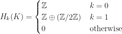
$H_0(S^1)=H_1(S^1)=\mathbb{Z}$ . Higher homology groups are zero.

$H_k(S^n)=\begin{cases}\mathbb{Z}&k=0,n\\ 0&\text{otherwise} \end{cases}$

$H_k(T)=\begin{cases}\mathbb{Z}\ \ \ &k=0,2\\ \mathbb{Z}\times\mathbb{Z}\ \ \ &k=1\\ 0\ \ \ &\text{otherwise} \end{cases}$

$H_k(\mathbb{R}P^2)=\begin{cases}\mathbb{Z}\ \ \ &k=0\\ \mathbb{Z}_2\ \ \ &k=1\\ 0\ \ \ &\text{otherwise} \end{cases}$

Klein bottle, $K$ : $H_k(K)=\begin{cases}\mathbb{Z}&k=0\\ \mathbb{Z}\oplus(\mathbb{Z}/2\mathbb{Z})&k=1\\ 0&\text{otherwise} \end{cases}$

Covering Spaces

A universal cover of a connected topological space $X$ is a simply connected space $Y$ with a map $f:Y\to X$ that is a covering map. Since there are many covering spaces, we will list the universal cover instead.

$\mathbb{R}$ is the universal cover of the unit circle $S^1$

$S^n$ is its own universal cover for $n>1$ . (General result: If $X$ is simply connected, i.e. has a trivial fundamental group, then it is its own universal cover.)

$\mathbb{R}^2$ is the universal cover of $T$ .

$S^2$ is universal cover of real projective plane $RP^2$ .

$\mathbb{R}^2$ is universal cover of Klein bottle $K$ .

ICM2014 (Seoul): Zhang YiTang

Math Online Tom Circle

ICM2014 (VideoSeries LC7):
Yitang Zhang

A conversation between Yitang Zhang and Daniel Goldston — who is one of the team GPY:

Simplified Prime Gap Video Explanations:

Video 1 – https://youtu.be/vkMXdShDdtY

Video 2 (extra) – https://youtu.be/D4_sNKoO-RA

View original post

“Proof School” For Math Kids

Math Online Tom Circle

To overcome the USA general school low Math standard, there are some elite schools to groom the gifted students such as this “Proof School”:

San-Fancisco new “Proof School” for Math kids
The Math Syllabus : Topology, Number Theory, …
IT: Python programming

Proof School Website
http://www.proofschool.org/#we-love-math

What is Proof School?

https://www.quora.com/What-is-Proof-School/answer/Alon-Amit?srid=oZzP&share=50c583a6

Math Syllabus:

http://www.proofschool.org/course-descriptions-1#math-courses

View original post

Interpolation Technique in Analysis

Question: Let $f$ belong to both $L^{p_1}$ and $L^{p_2}$ , with $1\leq p_1<p_2<\infty$ . Show that $f\in L^p$ for all $p_1\leq p\leq p_2$ .

There is a pretty neat trick to do this question, known as the “interpolation technique”. The proof is as follows.

For $p_1<p<p_2$ , there exists $0<\alpha<1$ such that $\displaystyle\boxed{p=\alpha p_1+(1-\alpha)p_2}$ . This is the key “interpolation step”. Once we have this, everything flows smoothly with the help of Holder’s inequality.

$\displaystyle\begin{aligned} \int |f|^p\ d\mu&=\int (|f|^{\alpha p_1}\cdot |f|^{(1-\alpha)p_2})\ d\mu\\ &\leq\||f|^{\alpha p_1}\|_\frac{1}{\alpha}\||f|^{(1-\alpha)p_2}\|_\frac{1}{1-\alpha}\\ &=(\int |f|^{p_1}\ d\mu)^\alpha\cdot (\int |f|^{p_2}\ d\mu)^{1-\alpha}\\ &<\infty \end{aligned}$

Thus $f\in L^p$ .

Note that the magical thing about the interpolation technique is that $p=\frac{1}{\alpha}$ and $q=\frac{1}{1-\alpha}$ are Holder conjugates, since $\frac{1}{p}+\frac{1}{q}=1$ is easily verified.

Undergraduate Math Books

Contractible space as Codomain implies any two maps Homotopic

Click here for: Free Personality Quiz

Recall that a space Y is contractible if the identity map $\text{id}_Y$ is homotopic to a constant map. Let Y be contractible space and let X be any space. Then, for any maps $f,g: X\to Y$ , $f\simeq g$ .

Proof: Let Y be a contractible space and let X be any space. $\text{id}_Y\simeq c$ , where $c$ is a constant map. There exists a map $F: Y\times [0,1]\to Y$ such that $F(y,0)=\text{id}_Y(y)=y$ , for $y\in Y$ . $F(y,1)=c(y)=b$ for some point $b\in Y$ .

Let $f,g: X\to Y$ be any two maps. Consider $G:X\times [0,1]\to Y$ where $G(x,t)=\begin{cases} F(f(x),2t),&\ \ \ \text{for}\ 0\leq t\leq 1/2\\ F(g(x),-2t+2),&\ \ \ \text{for}\ \frac 12<t\leq 1 \end{cases}$

When $t=\frac 12$ , $F(f(x),1)=b$ , $F(g(x),1)=b$ . Therefore G is cts.

$G(x,0)=F(f(x),0)=f(x)$ ,

$G(x,1)=F(g(x),0)=g(x)$ .

Therefore $f\simeq g$ .

Outer measure of Symmetric Difference Zero implies Measurability

Free Career Quiz: Please help to do!

Just came across this neat beginner’s Lebesgue Theory question. As students of analysis know, just to show a set is measurable is no easy feat. The usual way is to use the Caratheodory definition, where a set E is said to be measurable if for any set A, $m^*(A)=m^*(A\cap E)+m^*(A\cap E^c)$ . This can be quite tedious.

Question: Suppose E is a Lebesgue measurable set and let F be any subset of $\mathbb{R}$ such that $m^*(E\Delta F)=0$ (Symmetric Difference is Zero). Show that F is measurable.

The short way to do this is to note that $m^*(E\Delta F)=0$ implies $m^*(E\setminus F)=0$ , and $m^*(F\setminus E)=0$ . This in turn (using a lemma that any set with outer measure zero is measurable) implies the measurability of $E\setminus F$ and $\setminus F\setminus E$ .

Next comes the critical observation: $\boxed{E\cap F=E\setminus (E\setminus F)=E\cap (E\setminus F)^c}$ . Using the fact that the collection of measurable sets is a $\sigma$ -algebra, we can conclude $E\cap F$ is measurable.

Thus $F=(E\cap F)\cup (F\setminus E)$ is the union of two measurable sets and thus is measurable.

Interesting indeed!

Holder’s Inequality Trick

Click here: Free Career Quiz

Holder’s Inequality is a very useful inequality in Functional Analysis, hence many results can be proved by applying Holder’s Inequality.

Suppose that $\mu(\Omega)<\infty$ and $1\leq p_1<p_2\leq\infty$ . Prove that if $f_n\to f$ in $L^{p_2}$ , then $f_n\to f$ in $L^{p_1}$ .

Proof: Assume $f_n\to f$ in $L^{p_2}$ . Then there exists $N$ such that if $n\geq N$ , then $\|f_n-f\|_{p_2}=(\int |f_n-f|^{p_2} d\mu)^{1/p_2}<\epsilon$ .

Then, $\begin{aligned} \|f_n-f\|_{p_1}^{p_1}&=\int |f_n-f|^{p_1} d\mu\\ &=\||f_n-f|^{p_1}\cdot 1\|_1\\ &\leq\||f_n-f|^{p_1}\|_{p_2/p_1}\|1\|_{(p_2/p_1)'},\ \ \ \text{where } (p_2/p_1)'=\frac{p_2}{p_2-p_1}\ \text{is the Holder conjugate}\\ &=(\int |f_n-f|^{p_2}d\mu)^{p_1/p_2}(\int 1 d\mu)^\frac{p_2-p_1}{p_2}\\ &<\epsilon^{p_1}\cdot \mu(\Omega)^\frac{p_2-p_1}{p_2} \end{aligned}$

Since $\epsilon>0$ is arbitrary, $\|f_n-f\|_{p_1}^{p_1}\to 0$ as $n\to\infty$ .

Therefore, $\|f_n-f\|_{p_1}\to 0$ .

mu is countably additive if and only if it satisfies the Axiom of Continuity

Free Career Personality Quiz (Hundreds of people have tried it!)

Let $\mu$ be a finite, non-negative, finitely additive set function on a measurable space $(\Omega, \mathcal{A})$ . Show that $\mu$ is countably additive if and only if it satisfies the Axiom of Continuity: For $E_n\in\mathcal{A}, E_n\downarrow\emptyset \implies \mu(E_n)\to 0$ .

(=>) Assume $\mu$ is countably additive. Let $E_n\in\mathcal{A}$ , $E_n\downarrow\emptyset$ . Then,

$\displaystyle \lim_n \mu (E_n)=\mu (\cap_{n=1}^\infty E_n)=\mu (\emptyset)$ .

Suppose $\mu(\emptyset)=c$ . Then $\mu(\emptyset)=\mu(\cup_{n=1}^\infty \emptyset)=\sum_{n=1}^\infty c$ implies $c=0$ .

(<=) Assume $\mu$ satisfies Axiom of Continuity. Let $A_n\in\mathcal{A}$ be mutually disjoint sets. Define $E_n=\cup_{i=1}^\infty A_i\setminus \cup_{i=1}^n A_i$ .

Then $E_n\downarrow\emptyset$ . $\lim_n \mu(E_n)=0$ , $\lim_n \mu(\cup_{i=1}^\infty A_i)-\mu (\cup_{i=1}^n A_i)=0$ . $\lim_n \mu(\cup_{i=1}^n A_i)=\mu (\cup_{i=1}^\infty A_i)$ .

Therefore

$\begin{aligned}\mu(\cup_{i=1}^\infty A_i)&=\lim_n \mu(\cup_{i=1}^n A_i)\\ &=\lim_n \sum_{i=1}^n \mu (A_i)\\ &=\sum_{i=1}^\infty \mu(A_i) \end{aligned}$

Measure that is absolutely continuous with respect to mu

Interesting Career Personality Test (Free): https://mathtuition88.com/free-career-quiz/

Let $(X,\mathcal{M},\mu)$ be a measure space, and let $f:X\to [0,\infty]$ be a measurable function. Define the map $\lambda:\mathcal{M}\to[0,\infty]$ , $\lambda(E):=\int_X \chi_E f d\mu$ , where $\chi_E$ denotes the characteristic function of $E$ .

(a) Show that $\lambda$ is a measure and that it is absolutely continuous with respect to $\mu$ .

(b) Show that for any measurable function $g:X\to[0,\infty]$ , one has $\int_X g d\lambda=\int_X gf d\mu$ in $[0,\infty]$ .

Proof: For part (a), we routinely check that $\lambda$ is indeed a measure.

$\lambda(\emptyset)=\int_X \chi_\emptyset f d\mu=\int_X 0 d\mu=0$ . Let $E_i$ be mutually disjoiint measurable sets.

$\begin{aligned} \lambda(\cup_{i=1}^\infty E_i)&=\int_X \chi_{\cup_{i=1}^\infty E_i} f d\mu\\ &=\int_X (\sum_{i=1}^\infty \chi_{E_i}) f d\mu\\ &=\sum_{i=1}^\infty \int_X \chi_{E_i} f d\mu\\ &=\sum_{i=1}^\infty \lambda (E_i) \end{aligned}$

If $\mu (E)=0$ , then $\chi_{E} f=0$ a.e., thus $\lambda (E)=0$ . Therefore $\lambda\ll\mu$ .

(b) We note that when $g$ is a characteristic function, i.e. $g=\chi_E$ ,

$\begin{aligned} \int_X g d\lambda&=\int_X \chi_E d\lambda\\ &=\lambda (E)\\ &=\int_X \chi_E f d\mu\\ &=\int_X gf d\mu \end{aligned}$

Hence the equation holds. By linearity, we can see that the equation holds for all simple functions. Let $(\psi_n)$ be a sequence of simple functions such that $\psi_n\uparrow g$ . Then by the Monotone Convergence Theorem, $\lim_{n\to\infty} \int \psi_n d\lambda=\int g d\lambda$ .

Note that $\psi_n f\uparrow gf$ , thus by MCT, $\lim_{n\to\infty}\int\psi_n f d\mu=\int g f d\mu$ . Note that $\int \psi_n d\lambda=\int \psi_n f d\mu$ . Hence, $\int g d\lambda=\int gf d\mu$ , and we are done.

Interesting Analysis Question (Measure Theory)

Do try out this Free Career Guidance Personality Test at https://career-test.com/s/sgamb?reid=210 while it is still available!

Benefits of doing the (Free) Career Test:

Get familiar with the top companies in Singapore
There are seven distinct career types based on career preferences, goals and personality. Get to know yours! (My result: Harmonizer)
Take part in the annual Universum survey and win prizes!

Let $f\geq 0$ be a measurable function with $\int f d\mu<\infty$ . Show that for any $\epsilon>0$ , there exists a $\delta(\epsilon)>0$ such that for any measurable set $E\in\mathcal{A}$ with $\mu(E)<\delta(\epsilon)$ , we have $\int_E f d\mu<\epsilon$ .

Proof: For $M>0$ , we define $f_M(x)=\min (f(x),M)\leq M$ , for all $x\in \Omega$ .

Then $f=f_M+(f-f_M)$ .

Let $\delta=\epsilon/2M$ . Then for any $E\in\mathcal{A}$ with $\mu(E)<\delta$ ,

$\begin{aligned}\int_E f_M d\mu &\leq \int_E M d\mu\\ &=\mu (E)M\\ &<\delta M\\ &=(\epsilon/2M)M\\ &=\epsilon/2 \end{aligned}$

Note that $f_M\uparrow f$ . By Monotone Convergence Theorem,

$\int f d\mu=\lim_{M\to\infty}\int f_M d\mu$ .

Therefore $\lim_{M\to\infty}\int f-f_M d\mu=0$ .

We can choose $M$ sufficiently large such that

$\int_E f-f_M d\mu \leq \int f-f_M d\mu <\epsilon/2$ .

Then

$\begin{aligned} \int_E f d\mu&=\int_E f_M d\mu+\int_E f-f_M d\mu\\ &<\epsilon/2+\epsilon/2\\ &=\epsilon \end{aligned}$

We are done!

Zmn/Zm isomorphic to Zn

The following is a simple proof of why $\mathbb{Z}_{mn}/\mathbb{Z}_m\cong\mathbb{Z}_n$ .

For instance $\mathbb{Z}_6/\mathbb{Z}_2\cong\mathbb{Z}_3$ . Note that the tricky part is that $\mathbb{Z}_2$ is not actually the usual {0,1}, but rather {0,3} (considered as part of $\mathbb{Z}_6$ ). Hence the elements of $\mathbb{Z}_6/\mathbb{Z}_2$ are {0,3}, {1, 4}, {2, 5}, which can be seen to be isomorphic to $\mathbb{Z}_3$ .

A sketch of a proof is as follows. Consider $\phi:\mathbb{Z}_{mn}/\mathbb{Z}_m\to \mathbb{Z}_n$ , where $\mathbb{Z}_m=\{0,n,2n,\dots,(m-1)n\}$ , defined by $\phi (a+\mathbb{Z}_m)=a$ .

We may check that it is well-defined since if $a+\mathbb{Z}_m=a'+\mathbb{Z}_m$ , then $a\equiv a' \pmod n$ , and thus $\phi (a+\mathbb{Z}_m)=\phi (a'+\mathbb{Z}_m)$ .

It is a fairly straightforward to check it is a homomorphism, $\begin{aligned}\phi (a+\mathbb{Z}_m+a'+\mathbb{Z}_m)&=\phi (a+a'+\mathbb{Z}_m)\\ &=a+a'\\ &=\phi (a+\mathbb{Z}_m)+\phi(a'+\mathbb{Z}_m) \end{aligned}$

Injectivity is clear since $\ker \phi=0+\mathbb{Z}_m$ , and surjectivity is quite clear too.

Hence, this ends the proof. 🙂

Do check out some Recommended Books on Undergraduate Mathematics, and also download the free SG50 Scientific Pioneers Ebook, if you haven’t already.

Geometric n-simplex is convex

Given the definition of a geometric n-simplex:

$\displaystyle\sigma^n=\{x=\sum_{i=0}^{n}t_i a^i \mid t_i\geq 0\ \text{and }\sum_{i=0}^{n}=1\}\subseteq\mathbb{R}^n$

where $\{a^0,\dots, a^n\}$ are geometrically independent, we can show that the n-simplex is convex (i.e. given any two points, the line connecting them lies in the simplex).

Write $x=\sum_{i=0}^n t_i a^i$ , $y=\sum_{i=0}^n s_i a^i$ .

Consider the line from x to y: $\{ty+(1-t)x\mid 0\leq t\leq 1\}$ .

$\begin{aligned} ty+(1-t)x&=t\sum_{i=0}^n s_i a^i+(1-t)\sum_{i=0}^n t_i a^i\\ &=\sum_{i=0}^n (s_i t+t_i-tt_i)a_i\\ s_it+t_i-tt_i&=s_i t+t_i (1-t)\\ &\geq 0(0)+(0)(1-1)\\ &=0\\ \sum_{i=0}^n s_i t+t_i-tt_i &=t\sum_{i=0}^n s_i+\sum_{i=0}^n t_i -t\sum_{i=0}^n t_i\\ &=t(1)+(1)-t(1)\\ &=1 \end{aligned}$

Thus the line lies inside the simplex, and thus the simplex is convex.

Recommended Books for Math Majors

Cycle Decomposition of Permutations is Unique

Cycle decomposition of Permutations into disjoint cycles is unique (up to reordering of cycles).

A proof can be found here.

The condition of disjoint is crucial. For example, the permutation (1 3 2) can be factored into (2 3)(1 2), where the two cycles are not disjoint. (1 3 2)=(1 2)(1 3) is also another decomposition, the two cycles are also not disjoint.

Wolframalpha can calculate permutations, a useful tool to replace manual calculations. Take note though that Wolframalpha’s convention is multiplying permutations from left to right, while most books follow the convention of multiplying right to left.

Recommended Math Books from Amazon

Weierstrass M-test Proof and Special Case of Abel’s Theorem

First, let us recap what is Weierstrass M-test:

Weierstrass M-test:

Let $\{f_n\}$ be a sequence of real (or complex)-valued functions defined on a set A, and let $\{M_n\}$ be a sequence satisfying $\forall n\in\mathbb{N}, \forall x\in A$

$|f_n (x)|\leq M_n$ , and also $\sum_{n=1}^\infty M_n=M<\infty$ .

Then, $\sum_{n=1}^\infty f_n(x)$ converges uniformly on A (to a function f).

Proof:

Let $\epsilon >0$ . $\exists N\in\mathbb{N}$ such that $m\geq N$ implies $|M-\sum_{n=1}^m M_n|<\epsilon$ .

For $m\geq N, \forall x\in A$ ,

$\begin{aligned} |f(x)-\sum_{n=1}^m f_n(x)|&=|\sum_{n=m+1}^\infty f_n (x)|\\ &\leq\sum_{n=m+1}^\infty |f_n (x)|\\ &\leq \sum_{n=m+1}^\infty M_n\\ &=|M-\sum_{n=1}^m M_n|\\ &<\epsilon \end{aligned}$

Thus, $\sum_{n=1}^\infty f_n (x)$ converges uniformly.

Application to prove Abel’s Theorem (Special Case):

Consider the special case of Abel’s Theorem where all the coefficients $a_i$ are of the same sign (e.g. all positive or all negative).

Then, for $x\in [0,1]$ ,

$|a_n x^n|\leq |a_n|:=M_n$

Then by Weierstrass M-test, $\sum_{n=1}^\infty a_n x^n$ converges uniformly on [0,1] and thus $\lim_{x\to 1^-} \sum_{n=1}^\infty a_n x^n=\sum_{n=1}^\infty a_n$ .

Check out some books suitable for Math Majors here!

If Ratio Test Limit exists, then Root Test Limit exists, and both are equal

The limit for ratio test is $\lim_{n\to\infty} \frac{|a_{n+1}|}{|a_n|}$ , while the limit for root test is $\lim_{n\to\infty}|a_n|^{1/n}$ . Something special about these two limits is that if the former exists, the latter also exists and they are equal!

Proof:

Let $\lim_{n\to\infty}|\frac{a_{n+1}}{a_n}|=L$ . There exists $N\in\mathbb{N}$ such that $n\geq N \implies ||\frac{a_{n+1}}{a_n}|-L|<\epsilon$ .

i.e. $L-\epsilon<|\frac{a_{n+1}}{a_n}|<L+\epsilon$

For $n>N$ ,

$|a_n|=\frac{|a_n|}{|a_{n-1}|}\cdot \frac{|a_{n-1}|}{|a_{n-2}|}\cdots \frac{|a_{N+1}|}{|a_N|}\cdot |a_N| < (L+\epsilon)^{n-N}\cdot |a_N|$ .

Taking nth roots,

$|a_n|^{1/n}<(L+\epsilon)^\frac{n-N}{n}\cdot |a_N|^{\frac{1}{n}}$

Taking limits,

$\lim_{n\to\infty}|a_n|^{\frac{1}{n}}\leq (L+\epsilon)$

Since $\epsilon$ is arbitrary, $\lim_{n\to\infty}|a_n|^{\frac{1}{n}}\leq L$ .

Similarly, we can show $\lim_{n\to\infty}|a_n|^\frac{1}{n}\geq L$ .

Thus, $\lim_{n\to\infty}|a_n|^\frac{1}{n}=L$ .

This is considered a rather tricky (though not that difficult) proof, hope it helps whoever is searching for it!

Note that the converse is false, we can see that by considering the “rearranged” geometric series: 1/2,1, 1/8, 1/4, 1/32, … (source: https://www.maa.org/sites/default/files/0025570×33450.di021200.02p0190s.pdf)

where the ratio alternates from 2 to 1/8 and hence does not exist.

However, the root test limit of the first 2n terms is defined:

$\begin{aligned} |a_{2n}|&=\frac{|a_{2n}|}{a_{2n-1}}\cdot \frac{|a_{2n-1}|}{|a_{2n-2}|}\cdot \frac{|a_2|}{|a_1|}\cdot |a_1|\\ &=2\cdot \frac{1}{8}\cdot 2 \cdot \frac{1}{8} \cdots 2 \cdot \frac{1}{2}\\ &=2^n \cdot (\frac{1}{8})^{n-1}\cdot \frac{1}{2}\\ &=(\frac{1}{4})^{n-1} \end{aligned}$

Thus, $|a_{2n}|^\frac{1}{2n}=\frac{1}{4}^{\frac{n-1}{2n}}\to \frac{1}{2}$ .

To learn more about epsilon-delta proofs, check out one of the Recommended Analysis Books for Undergraduates.

Z[Sqrt(-2)] is a Principal Ideal Domain Proof

It turns out that to prove $\mathbb{Z}[\sqrt{-2}]$ is a Principal Ideal Domain, it is easier to prove that it is a Euclidean domain, and hence a PID.

(Any readers who have a direct proof that $\mathbb{Z}[\sqrt{-2}]$ is a PID, please comment below, as it would be very interesting to know such a proof. 🙂 )

Proof:

As mentioned above, we will prove that it is a Euclidean domain.

Let $a, b\in\mathbb{Z}[\sqrt{-2}], b\neq 0$ .

We need to show: $\exists q, r\in \mathbb{Z}[\sqrt{-2}]$ such that $a=bq+r$ , with $N(r)<N(b)$ .

Consider $\frac{a}{b}=c_1+c_2 \sqrt{-2} \in \mathbb{Q}[\sqrt{-2}]$ . Define $q=q_1+q_2 \sqrt{-2}$ where $q_1, q_2$ are the integers closest to $c_1, c_2$ respectively.

Then, $\frac{a}{b}=q+\alpha$ , where $\alpha=\alpha_1+\alpha_2 \sqrt{-2}$ .

$a=bq+b\alpha$ .

Take $r=b\alpha$ .

$\begin{aligned} N(r)&=N(b\alpha)\\ &=N(b)\cdot N(\alpha)\\ &=N(b)\cdot (\alpha_1^2+2\alpha_2^2)\\ &\leq N(b)\cdot ({\frac{1}{2}}^2+2(\frac{1}{2})^2)\\ &=N(b)\cdot (\frac{3}{4})\\ &<N(b) \end{aligned}$

Check out recommended Abstract Algebra books: Recommended Books for Math Undergraduates

Definition of Euclidean Domain and Principal Ideal Domain (PID)

A Euclidean domain is an integral domain $R$ with a function $d:R\setminus \{0\}\to \mathbb{N}$ satisfying the following:

(1) $d(a)\leq d(ab)$ for all nonzero $a,b$ in $R$ .

(2) for all $a,b \in R$ , $b\neq 0$ , $\exists q, r, \in R$ such that $a=bq+r$ , with either $r=0$ or $d(r)<d(b)$ .

(d is known as the Euclidean function)

On the other hand, a Principal ideal domain (PID) is an integral domain in which every ideal is principal (can be generated by a single element).

Allot more time for exam papers (Straits Times Forum)

Source: http://www.straitstimes.com/forum/letters-on-the-web/allot-more-time-for-exam-papers

This reader has called for allotting more time for exam papers. He/she has made a very valid point:

The time allotted for some papers, such as mathematics, is so limited that the opportunity cost of stopping for just a few minutes to think about how to solve a problem may result in one being unable to complete the paper.

For essay papers in subjects such as economics, it becomes a test of how fast one can write, as opposed to the quality of one’s answers.

This is very true, the reader is being 100% honest and not exaggerating at all! For O Levels and A Levels Maths, the student can only spend 1.5min per mark. That means, for a 5 mark long question, he can only spend 7.5 min at the maximum or risk not being able to finish the paper. To have ample time to check the paper, the student needs to do even faster than the minimum of 1.5 min per mark.

Yoda’s quote “Do. Or do not. There is no try.” holds true for Mathematics exam papers in Singapore. There is simply no time to “try” out questions in O Level or A Level Maths. Once a student looks at the question, his fate is sealed, he/she either knows the method how to do it, or does not. There is no time to try!

Hence, exam time management skills and speed in Math are essential. (I have written a previous post about it.) Nowadays, questions are not arranged in order of difficulty. This means that Question 5 may be much harder than Question 10. Sometimes, it is better to skip Question 5, rather than get stuck on it and never reach Question 10. Getting 100% is not necessary for getting an A for Math. In fact, getting 100% for Math after Primary 6 is a rare occurrence. Getting 70 for Math in H2 Math is a very decent score, and getting 80 more or less guarantees an A even with a bell curve.

Also, knowledge of the essential formulas are extremely important. Yes, it is possible to derive the quadratic formula by completing the square, but there is no time for that during the exam. Time is of essence. Formula for AP/GP, Vectors need to be known by heart. Spending 1 min to recall or derive them may lead to severe time pressure later on. Recalling the wrong formula leads to disaster, and potentially zero marks for the entire question, as “error carry forward” is only applicable for limited scenarios. Students may need a Formula Helpsheet containing all the essential formulas for easy memorization.

Lastly, the most important thing the night before the exam is have a good night’s sleep. A previous blog post discusses the importance of sleep, and how Good night’s sleep adds up to better exam results – especially in maths. Also, have a good rest after the Math paper, the 3 hour H2 paper is mentally exhausting, and the 2.5 hour A Maths paper is not a stroll in the park either. After the long Maths paper, your brain deserves a good rest.

Proof of Associativity of Operation * on Path-homotopy Classes

(Continued from https://mathtuition88.com/2015/06/25/the-groupoid-properties-of-operation-on-path-homotopy-classes-proof/)

Earlier we have proved the properties (2) Right and left identities, (3) Inverse, leaving us with (1) Associativity to prove.

For this proof, it will be convenient to describe the product f*g in the language of positive linear maps.

First we will need to define what is a positive linear map. We will elaborate more on this since Munkres’ books only discusses it briefly.

Definition: If [a,b] and [c,d] are two intervals in $\mathbb{R}$ , there is a unique map $p:[a,b]\to [c.d]$ of the form p(x)=mx+k that maps a to c and b to d. This is called the positive linear map of [a,b] to [c,d] because its graph is a straight line with positive slope.

Why is it a positive slope? (Not mentioned in the book) It turns out to be because we have:

p(a) = ma+k=c

p(b) = mb+k=d

Hence, d-c = mb-ma = m(b-a)

Thus, m=(d-c)/(b-a), which is positive since d-c and b-a are all positive quantities.

Note that the inverse of a positive linear map is also a positive linear map, and the composite of two such maps is also a positive linear map.

Now, we can show that the product f*g can be described as follows: On [0,1/2], it is the positive linear map of [0,1/2] to [0,1], followed by f; and on [1/2,1] it equals the positive linear map of [1/2,1] to [0,1], followed by g.

Let’s see why this is true. The positive linear map of [0,1/2] to [0,1] is p(x)=2x. fp(x) = f(2x).

The positive linear map of [1/2,1] to [0,1] is p(x)=2x-1. gp(x)=g(2x-1).

If we look back at the earlier definition of f*g, that is precisely it!

Now, given paths, f, g, and h in X, the products f*(g*h) and (f*g)*h are defined if and only if f(1)=g(0) and g(1)=h(0), i.e. the end point of f = start point of g, and the end point of g = start point of h. If we assume that these two conditions hold, we can also define a triple product of the paths f, g, and h as follows:

Choose points a and b of I so that 0<a<b<1. Define a path $k_{a,b}$ in X as follows: On [0,a] it equals the positive linear map of [0,a] to I=[0,1] followed by f; on [a,b] it equals the positive linear map of [a,b] to I followed by g; on [b,1] it equals the positive linear map of [b,1] to I followed by h. This path $k_{a,b}$ depends on the choice of the values of a and b, but its path-homotopy class turns out to be independent of a and b.

We can show that if c and d are another pair of points of I with 0<c<d<1, then $k_{c,d}$ is path homotopic to $k_{a,b}$ .

Let $p:I\to I$ be the map whose graph is pictured in Figure 51.9 (taken from Munkre’s Book)

On the intervals [0,a], [a,b], [b,1], it equals the positive linear maps of these intervals onto [0,c],[c,d],[d,1] respectively. It follows that $k_{c,d} \circ p = k_{a,b}$ . Let’s see why this is so.

On [0,a] $k_{c,d}\circ p$ is the positive linear map of [0,a] to [0,c], followed by the positive linear map of [0,c] to I, followed by f. This equals the positive linear map of [0,a] to I, followed by f, which is precisely $k_{a,b}$ . Similar logic holds for the intervals [a,b] and [b,1].

$p$ is a path in I from 0 to 1, and so is the identity map $i: I\to I$ . Since I is convex, there is a path homotopy P in I between p and i. Then, $k_{c,d}\circ P$ is a path homotopy in X between $k_{a,b}$ and $k_{c.d}$ .

Now the question many will be asking is: What has this got to do with associativity. According to the author Munkres, “a great deal”! We check that the product $f*(g*h)$ is exactly the triple product $k_{a,b}$ in the case where $a=1/2$ and $b=3/4$ .

By definition,

$(g*h)(s)=\begin{cases} g(2s)\ &\text{for }s\in [0,\frac{1}{2}]\\ h(2s-1)\ &\text{for }s\in [\frac{1}{2},1] \end{cases}$

Thus, $f*(g*h)(s)=\begin{cases} f(2s)\ &\text{for }s\in [0,\frac{1}{2}]\\ (g*h)(2s-1)\ &\text{for }s\in [\frac{1}{2},1] \end{cases} =\begin{cases} f(2s)\ &\text{for }s\in [0,\frac{1}{2}]\\ g(4s-2)\ &\text{for }s\in [\frac{1}{2},\frac{3}{4}]\\ h(4s-3) &\text{for }s\in [\frac{3}{4},1] \end{cases}$

We can also check in a very similar way that $(f*g)*h)=k_{c,d}$ when c=1/4 and d=1/2. Thus, the these two products are path homotopic, and we have finally proven the associativity of *.

Reference:

Topology (2nd Economy Edition)

“I LOVE YOU” Math Graph

This is how to plot “I LOVE YOU” using Math Graphs (many piecewise functions plotted together).

Interesting? Share it using the buttons below this post!

Source: Found it on Weibo (China’s version of Facebook)

Love and Math: The Heart of Hidden Reality

What if you had to take an art class in which you were only taught how to paint a fence? What if you were never shown the paintings of van Gogh and Picasso, weren’t even told they existed? Alas, this is how math is taught, and so for most of us it becomes the intellectual equivalent of watching paint dry.

In Love and Math, renowned mathematician Edward Frenkel reveals a side of math we’ve never seen, suffused with all the beauty and elegance of a work of art. In this heartfelt and passionate book, Frenkel shows that mathematics, far from occupying a specialist niche, goes to the heart of all matter, uniting us across cultures, time, and space.

Lemma on Measure of Increasing Sequences in X

(Continued from https://mathtuition88.com/2015/06/20/what-is-a-measure-measure-theory/)

Lemma: Let $\mu$ be a measure defined on a $\sigma$ -algebra X.

(a) If ( $E_n$ ) is an increasing sequence in X, then

$\mu (\bigcup_{n=1}^\infty E_n )=\lim \mu (E_n)$

(b) If $F_n$ ) is a decreasing sequence in X and if $\mu (F_1)<\infty$ , then

$\mu (\bigcap_{n=1}^\infty F_n )=\lim \mu (F_n )$

Note: An increasing sequence of sets ( $E_n$ ) means that for all natural numbers n, $E_n \subseteq E_{n+1}$ . A decreasing sequence means the opposite, i.e. $E_n \supseteq E_{n+1}$ .

Proof: (Elaboration of the proof given in Bartle’s book)

(a) First we note that if $\mu (E_n) = \infty$ for some n, then both sides of the equation are $\infty$ , and inequality holds. Henceforth, we can just consider the case $\mu (E_n)<\infty$ for all n.

Let $A_1 = E_1$ and $A_n=E_n \setminus E_{n-1}$ for n>1. Then $(A_n)$ is a disjoint sequence of sets in X such that

$E_n=\bigcup_{j=1}^n A_j$ , $\bigcup_{n=1}^\infty E_n = \bigcup_{n=1}^\infty A_n$

Since $\mu$ is countably additive,

$\mu (\bigcap_{n=1}^\infty E_n) = \sum_{n=1}^\infty \mu (A_n)$ (since ( $A_n$ ) is a disjoint sequence of sets)

$=\lim_{m\to\infty} \sum_{n=1}^m \mu (A_n)$

By an earlier lemma $\mu (F\setminus E)=\mu (F)-\mu (E)$ , we have that $\mu (A_n)=\mu (E_n)-\mu (E_{n-1})$ for n>1, so the finite series on the right side telescopes to become

$\sum_{n=1}^m \mu (A_n)=\mu (E_m)$

Thus, we indeed have proved (a).

For part (b), let $E_n=F_1 \setminus F_n$ , so that $(E_n)$ is an increasing sequence of sets in X.

We can then apply the results of part (a).

$\begin{aligned} \mu (\bigcup_{n=1}^\infty E_n) &=\lim \mu (E_n)\\ &=\lim [\mu (F_1)-\mu (F_n)]\\ &=\mu (F_1) -\lim \mu (F_n) \end{aligned}$

Since we have $\bigcup_{n=1}^\infty E_n =F_1 \setminus \bigcap_{n=1}^{\infty} F_n$ , it follows that

$\mu (\bigcup_{n=1}^\infty E_n) =\mu (F_1)-\mu (\bigcap_{n=1}^\infty F_n)$

Comparing the above two equations, we get our desired result, i.e. $\mu (\bigcap_{n=1}^\infty F_n) = \lim \mu (F_n)$ .

Reference:

The Elements of Integration and Lebesgue Measure

What is a Measure? (Measure Theory)

In layman’s terms, “measures” are functions that are intended to represent ideas of length, area, mass, etc. The inputs for the measure functions would be sets, and the output would be a real value, possibly including infinity.

It would be desirable to attach the value 0 to the empty set $\emptyset$ and measures should be additive over disjoint sets in X.

Definition (from Bartle): A measure is an extended real-valued function $\mu$ defined on a $\sigma$ -algebra X of subsets of X such that
(i) $\mu (\emptyset)=0$
(ii) $\mu (E) \geq 0$ for all $E\in \mathbf{X}$
(iii) $\mu$ is countably additive in the sense that if $(E_n)$ is any disjoint sequence ( $E_n \cap E_m =\emptyset\ \text{if }n\neq m$ ) of sets in X, then

$\displaystyle \mu(\bigcup_{n=1}^\infty E_n )=\sum_{n=1}^\infty \mu (E_n)$ .

If a measure does not take on $+\infty$ , we say it is finite. More generally, if there exists a sequence $(E_n)$ of sets in X with $X=\cup E_n$ and such that $\mu (E_n) <+\infty$ for all n, then we say that $\mu$ is $\sigma$ -finite. We see that if a measure is finite implies it is $\sigma$ -finite, but not necessarily the other way around.

Examples of measures

(a) Let X be any nonempty set and let X be the $\sigma$ -algebra of all subsets of X. Let $\mu_1$ be definied on X by $\mu_1 (E)=0$ , for all $E\in\mathbf{X}$ . We can see that $\mu_1$ is finite and thus also $\sigma$ -finite.

Let $\mu_2$ be defined by $\mu_2 (\emptyset) =0$ , $\mu_2 (E)=+\infty$ if $E\neq \emptyset$ . $\mu_2$ is an example of a measure that is neither finite nor $\sigma$ -finite.

The most famous measure is definitely the Lebesgue measure. If X=R, and X=B, the Borel algebra, then (shown in Bartle’s Chapter 9) there exists a unique measure $\lambda$ defined on B which coincides with length on open intervals. I.e. if E is the nonempty interval (a,b), then $\lambda (E)=b-a$ . This measure is usually called Lebesgue measure (or sometimes Borel measure). It is not a finite measure since $\lambda (\mathbb{R})=\infty$ . But it is $\sigma$ -finite since any interval can be broken down into a sequence of sets ( $E_n$ ) such that $\mu (E_n)<\infty$ for all n.

Source: The Elements of Integration and Lebesgue Measure

5-21-1471

Albrecht Durer, the German painter and engraver who studied mathematics and applied it to his art, was born in Nuremberg on this day.

More information about:

Albrecht Durer

from On This Day http://ift.tt/1HiQ6Mx
via IFTTT

Recommended Tuition Agency:

Startutor is Singapore’s most popular online agency, providing tutors to your home. There are no extra costs for making a request. The tutors’ certificates are carefully checked by Startutor. (Website: http://ift.tt/1HiQ33b) There are many excellent tutors from RI, Hwa Chong, etc. at Startutor, teaching various subjects at all levels. High calibre scholars from NUS/overseas universities are also tutoring at Startutor. (Website: http://ift.tt/1HiQ33b) (Please use the full link above directly, thanks!)

Chinese Tuition: http://ift.tt/1JvQvA2

Math Resources / Short, Summarized Math Notes for Sale: http://ift.tt/1HiQ0oa 10% Discount on all products (Free Exam Papers from Top Schools to accompany each Math Resource.) Recommended Books for GEP: http://ift.tt/1HiQ0Eo Singapore Math Books: http://ift.tt/1OpA3mw

5-21-1923

Armand Borel born in Switzerland. He worked on Lie groups, algebraic groups, and arithmetic groups, helping transform many areas of mathematics, including algebraic topology, differential geometry, algebraic geometry, and number theory.

More information about:

Armand Borel

from On This Day http://ift.tt/1HiQ3QS
via IFTTT

Recommended Tuition Agency:

Chinese Tuition: http://ift.tt/1JvQvA2

5-21-1953

Set theorist Ernst Zermelo died in Freiburg, Germany. He worked on statistical mechanics and the calculus of variations until becoming intrigued by Cantor’s Continuum Hypothesis, posed as Hilbert’s First Problem in 1900, and switching to set theory.

More information about:

Ernst Zermelo

from On This Day http://ift.tt/1AmxuOk
via IFTTT